Surplus production models
Surplus production models for data-poor species
VAST includes features to track fishing mortality F_ct for each category and year. A 1st order autoregressive process using a log-linked Poisson or Tweedie distribution (or alternatively a Poisson-linked delta model) is equivalent to Gompertz density dependence, and it is then possible to track the net effect of past and present fishing mortality on current biomass, as well as calculate biomass and fishing mortality reference points (the latter using “spawning potential ratio” F_%SPR metrics).
We show this process in an example below for Gulf of Alaska pollock. We note that initial fits yielded an implausible value for autocorrelation (and resulting fishing mortality targets). We have therefore taken the F_40% = 0.281 from the 2019 stock assessment and back-calculated the resulting magnitude of first-order autocorrelation, Rho = 0.69. We then fixed this value during model fits.
This approach could be substantially extended in future applications. For example:
- The current approach inputs a fishing mortality
F_ct, e.g., from a time-series of fishing effort and assumed catchability coefficient within an area-swept estimator. Future developments could instead fit to annual catch data. - The software implementation does not allow autocorrelation in both intercepts
betaand spatio-temporal variationepsilon, but this could easily be changed.
For more details see e.g.
- An extended version with movement
- An extended multi-species version
library(VAST)
example = load_example( "GOA_MICE_example" )

# Get settings
settings = make_settings( n_x=50,
  purpose="index2",
  Region=example$Region,
  n_categories = 1,
  max_cells = 5000,
  Options = c(Calculate_Fratio=TRUE, Estimate_B0=TRUE),
  vars_to_correct = c("Index_ctl","Bratio_ctl") )

# Modify defaults
settings$RhoConfig = c("Beta1"=3, "Beta2"=3, "Epsilon1"=4, "Epsilon2"=6)
settings$FieldConfig[] = 1

# Subset MICE-in-space example data
sampling_data = subset(example$sampling_data, spp=="Gadus_chalcogrammus")
sampling_data$spp = droplevels(sampling_data$spp)
F_ct = example$F_ct['POLLOCKWCWYK2016',,drop=FALSE]

# Build initial model
Inputs = fit_model( settings = settings,
  Lat_i = sampling_data[,'Lat'],
  Lon_i = sampling_data[,'Lon'],
  b_i = sampling_data[,'Catch_KG'],
  a_i = sampling_data[,'AreaSwept_km2'],
  t_i = sampling_data[,'Year'],
  F_ct = F_ct,
  build_model = FALSE )

# Map off 1st order autocorrelation
  # and fix at value implied by F_40 SPR target given Gompertz dynamics
# F_40 = 0.281
Map = Inputs$tmb_list$Map
  Map$Epsilon_rho1_f = factor(NA)
Params = Inputs$tmb_list$Parameters
  Params$Epsilon_rho1_f = 1 - (0.281 / (-1 * log(0.4)))

# Run initial model
fit = fit_model( settings = settings,
  Lat_i = sampling_data[,'Lat'],
  Lon_i = sampling_data[,'Lon'],
  b_i = sampling_data[,'Catch_KG'],
  a_i = sampling_data[,'AreaSwept_km2'],
  t_i = sampling_data[,'Year'],
  F_ct = F_ct,
  Map = Map,
  Parameters = Params,
  getsd = TRUE,
  year_labels = c(1975, 1984:2015) )

# Fix issue in auto-generated plot labels
fit$years_to_plot = 1:length(fit$year_labels)  # Plot all years, not just years with samples

# Plots
plot_results( fit = fit,
  settings = settings,
  check_residuals = FALSE,
  country = "united states of america",
  use_new_epsilon = FALSE,
  mfrow = c(9,4) )
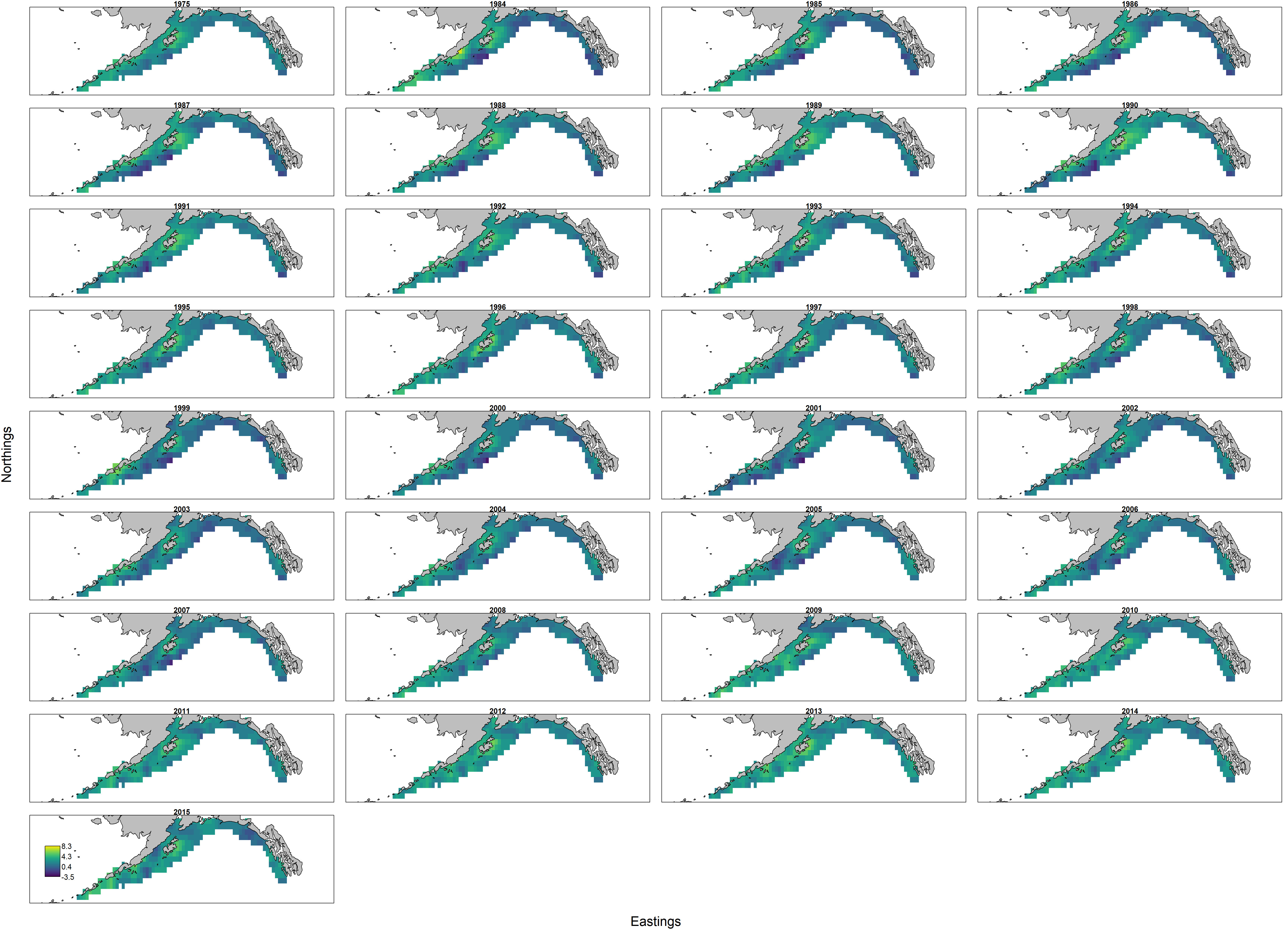
Inspecting the density maps shows:
- that the model is now estmating a initial biomass (labeled as 1975 above), representing predicted biomass in the absence of fishing;
- the model interpolates densities and abundance even in years without survey data, based on the autocorrelation derived from the SPR target as well as intervening fishing mortality.
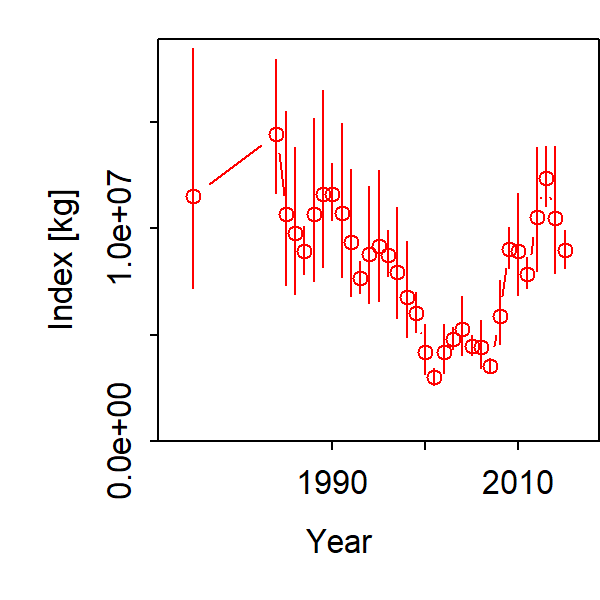
Inspecting the abundance index we see substantial uncertainty about initial biomass (labeled as 1975), followed by a decline and recovery in total biomass:
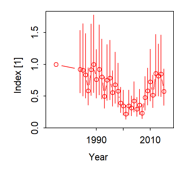
We can also compute the total biomass relative to the mean of it’s stationary value in the absence of fishing, which we call B0. This ratio is often called depletion:
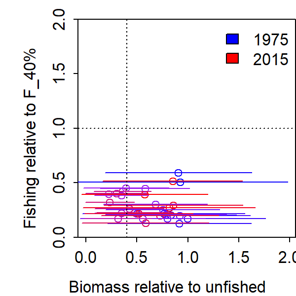
Finally, we can plot depletion against the inputted fishing mortality relative to the assumed F_40 reference point, which we call exploitation rate. This ratio is known exactly, because it is composed of an inputted fishing mortality and reference point. However, calculating this relative to depletion provides a plot of estimated “stock status”.