Modelling densities along a stream network
Stream network models
Users can fit VAST to data arising along a stream-network, and this can be done in combination with any other feature available in VAST.
In the following, we specifically use data for longfin eel in New Zealand, and define an object network that defines a directed acyclic graph representing the stream network. The example below is based upon the case-study from Charsley et al. 2023, and thanks for A. Charsley, M. Rudd, A. Gruss and many others who contributed to developing the stream-network features and code.
In the future, we hope to improve the output/output interface, and please email the package developers for more information.
#
library(VAST)
library(tidyverse)

#Load data
data <- data("stream_network_eel_example")

#Set stream network, observations and habitat data
network <- stream_network_eel_example[["network"]]   #stream network
obs <- stream_network_eel_example[["observations"]]  #longfin eel presence/absence data

#Only using electric fishing and net/trap data
obs <- obs %>% filter(fishmethod %in% c("Electric fishing", "Net", "Trap"))

#Combine net and trap methods to reduce number of catchability parameters estimated
obs$fishmethod <- ifelse(obs$fishmethod %in% c("Net", "Trap"), "Net_trap",
                         ifelse(obs$fishmethod == "Electric fishing", "Electric fishing", NA))

#Extract stream network data for VAST model
Network_sz = network %>% select(c('parent_s','child_s','dist_s'))
Network_sz_LL = network %>% select(c('parent_s','child_s','dist_s','Lat','Lon'))

#Setup dataset
Data_Geostat <- data.frame( "Catch_KG" = obs$data_value,
                            "Year" = obs$year,
                            "Fishing_method" = obs$fishmethod,
                            "Sampler" = obs$agency,
                            "AreaSwept_km2" = obs$dist_i,
                            "Lat" = obs$lat,
                            "Lon" = obs$long,
                            "Child_i" = obs$child_i)

#Add a small value to presence observations - needed for binomial models
set.seed(22)
Data_Geostat[,'Catch_KG'] = Data_Geostat[,'Catch_KG'] * exp(1e-3*rnorm(nrow(Data_Geostat)))

#Set up catchability effects
Q1_formula <- ~ Fishing_method
Q1config_k <- 1
#Q2_formula <- ~ 0
#Q2config_k <- NULL
catchability_data <- Data_Geostat[,c("Lat", "Lon", "Fishing_method")]

#set up example model configuration
FieldConfig = c("Omega1"=1, "Epsilon1"=1, "Omega2"=0, "Epsilon2"=0)
RhoConfig = c("Beta1"=2, "Beta2"=3, "Epsilon1"=0, "Epsilon2"=0)
ObsModel = cbind("PosDist"=2,"Link"=0)
Options =  c("Calculate_Range"=1,
             "Calculate_effective_area"=1)
#Settings
settings <- make_settings(n_x = nrow(Network_sz),
                          purpose = "index2",
                          Region = "Stream_network",
                          fine_scale = FALSE,
                          FieldConfig = FieldConfig,
                          RhoConfig = RhoConfig,
                          ObsModel = ObsModel,
                          bias.correct = F,
                          Options = Options)
settings$Method <- "Stream_network"
settings$grid_size_km <- 1

#Run model
fit = fit_model( settings=settings,
                 Lat_i=Data_Geostat[,"Lat"],
                 Lon_i=Data_Geostat[,"Lon"],
                 t_i=as.numeric(Data_Geostat[,'Year']),
                 b_i=Data_Geostat[,'Catch_KG'],
                 a_i=Data_Geostat[,'AreaSwept_km2'],
                 catchability_data = catchability_data,
                 Q1_formula = Q1_formula,
                 Q2_formula = Q2_formula,
                 Q1config_k = Q1config_k,
                 Q2config_k = Q2config_k,
                 input_grid=cbind( "Lat"=Data_Geostat[,"Lat"],
                                   "Lon"=Data_Geostat[,"Lon"],
                                   "Area_km2"=Data_Geostat[,"AreaSwept_km2"],
                                   "child_i"=Data_Geostat[,"Child_i"]),
                 Network_sz_LL=Network_sz_LL,
                 Network_sz = Network_sz)
We can then visulize outputs using conventional VAST plots, or can save the object and re-plot using ggplot:
#Plot results
plot_results( fit=fit,
category_names="Longfin eels",
plot_set=c(1,6),
land_color = rgb(1,1,1,0.2) )
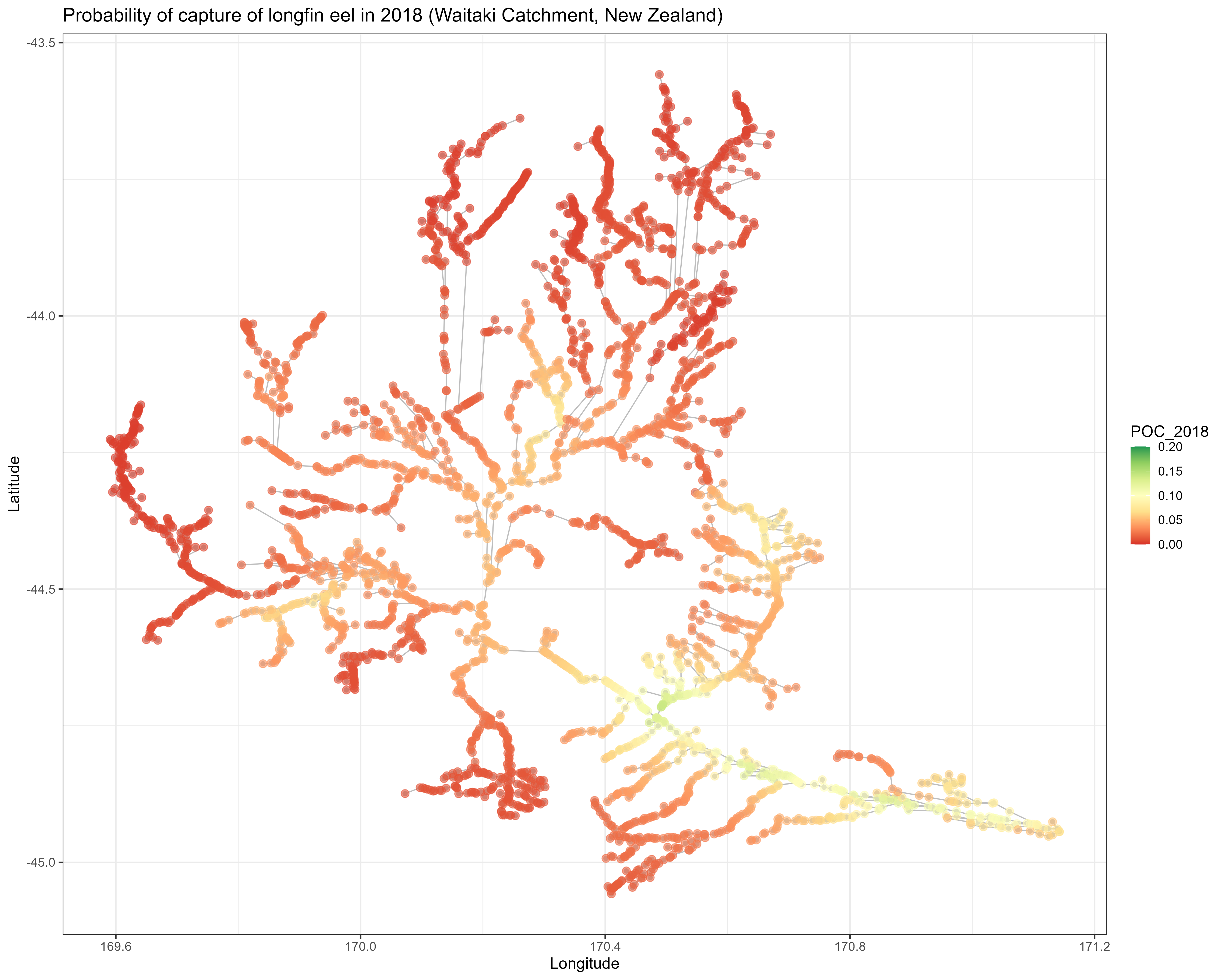
#Probability of capture estimates
POC <- matrix(fit$Report$R1_gct[,1,], ncol = 59, dimnames = list(network$child_s, min(Data_Geostat$Year):max(Data_Geostat$Year)))
POC_df <- data.frame("Lat" = network$Lat, "Lon"=network$Lon, "POC_2018"=POC[,"2018"]) #2018 is the latest year in dataset
#Catchment tracing
l2 <- lapply(1:nrow(network), function(x){
parent <- network$parent_s[x]
find <- network %>% filter(child_s == parent)
if(nrow(find)>0) out <- cbind.data.frame(network[x,], 'Lon2'=find$Lon, 'Lat2'=find$Lat)
if(nrow(find)==0) out <- cbind.data.frame(network[x,], 'Lon2'=NA, 'Lat2'=NA)
return(out)
})
l2 <- do.call(rbind, l2)
#Plot POC in catchment
catchmap <- ggplot(POC_df) +
geom_point(data = network, aes(x = Lon, y = Lat), col = "gray") +
geom_segment(data=l2, aes(x = Lon2,y = Lat2, xend = Lon, yend = Lat), col="gray") +
geom_point(aes(x = Lon, y = Lat, col = POC_2018), size=3, alpha = 0.6) +
xlab("Longitude") + ylab("Latitude") +
ggtitle("Probability of capture of longfin eel in 2018 (Waitaki Catchment, New Zealand)") +
scale_color_distiller(palette = "RdYlGn", limits = c(0,0.2), direction = 1) +
theme_bw(base_size = 14) +
theme(axis.text = element_text(size = rel(0.8)))
Works cited
Charsley, A. R., Grüss, A., Thorson, J. T., Rudd, M. B., Crow, S. K., David, B., Williams, E. K., & Hoyle, S. D. (2023). Catchment-scale stream network spatio-temporal models, applied to the freshwater stages of a diadromous fish species, longfin eel (Anguilla dieffenbachii). Fisheries Research, 259, 106583. https://doi.org/10.1016/j.fishres.2022.106583
Hocking, D. J., Thorson, J. T., O’Neil, K., & Letcher, B. H. (2018). A geostatistical state-space model of animal densities for stream networks. Ecological Applications, 28(7), 1782–1796. https://doi.org/10.1002/eap.1767