Empirical Orthogonal Function (EOF) analysis for biological data
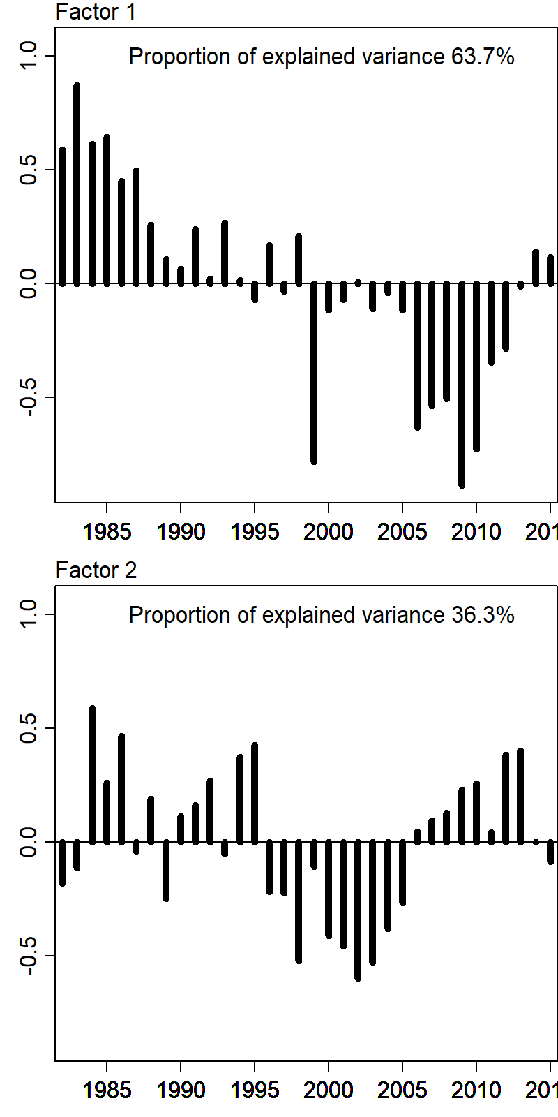
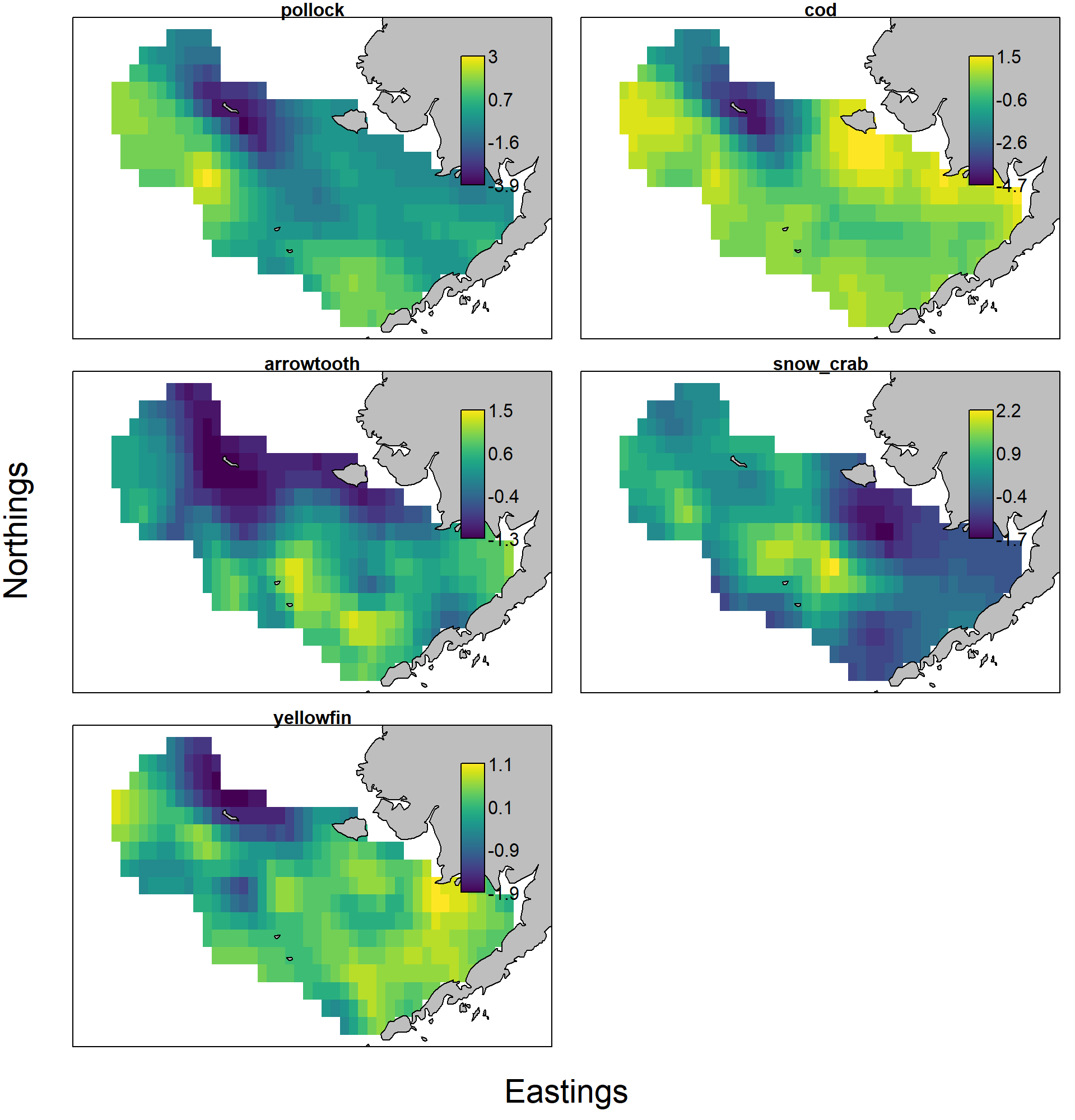
It is possible to use VAST to fit a generalization of empirical orthogonal function (EOF) analysis, while accounting for the noisy, zero-inflated and multivariate data that we have in fisheries. To do so, take a univariate or multivariate model and perform rank-reduction (a.k.a. ordination) on years; this contrasts with “conventional” joint dynamic species distribution models, which ordinate on species. In this case, the model will then estimate spatial variability for each species, one or more annual indices of variability, as well a map for each mode and species indicating the deviation from uniform distribution associated with a positive value of each index for each species. It is possible to visualize the statistical significance of each model component, e.g., to visualize whether index variability is “significant” or to identify locations that are “significantly” associated with a given index.
In this example, we apply EOF to five groundfishes in the eastern Bering Sea. This was initially explored and documented in Thorson Ciannelli & Litzow (2020).
Example code
# Load packages
library(VAST)

# load data set
example = load_example( data_set="five_species_ordination" )

# Make settings:
# including modifications from default settings to match
# analysis in original paper
settings = make_settings( n_x=50,
  Region=example$Region,
  purpose="EOF3",
  n_categories=2,
  ObsModel=c(1,1),
  RhoConfig=c("Beta1"=0,"Beta2"=0,"Epsilon1"=0,"Epsilon2"=0) )

# Run model (including settings to speed up run)
fit = fit_model( settings=settings,
  Lat_i=example$sampling_data[,'Lat'],
  Lon_i=example$sampling_data[,'Lon'],
  t_i=example$sampling_data[,'Year'],
  c_i=example$sampling_data[,'species_number']-1,
  b_i=example$sampling_data[,'Catch_KG'],
  a_i=example$sampling_data[,'AreaSwept_km2'],
  newtonsteps=0,
  getsd=FALSE,
  Use_REML=TRUE )

# Plot results, including spatial term Omega1
results = plot( fit,
  check_residuals=FALSE,
  plot_set=c(3,16),
  category_names = c("pollock", "cod", "arrowtooth", "snow_crab", "yellowfin") )
The 2nd index is highly correlated with the cold-pool extent:
and the estimated response maps show the expected response for pollock and cod, e.g., where a year with large cold-pool extent has decreased densities in the northern portion of the eastern Bering Sea:
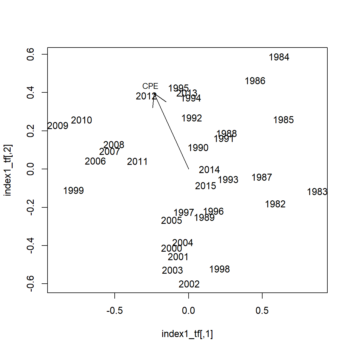
We can further explore these patterns by visualizing factor loadings in in relation to the cold-pool extent:
# Load Cold-pool-extent
example2 = load_example( data_set="EBS_pollock" )
CPE = example2$covariate_data[match(fit$year_labels,example2$covariate_data$Year),'AREA_SUM_KM2_LTE2']
# use `ecodist` to display ordination
index1_tf = results$Factors$Rotated_loadings$EpsilonTime1
cpe_vf = ecodist::vf(index1_tf, data.frame("CPE"=CPE), nperm=1000)
png( "year_ordination.png", width=6, height=6, res=200, units="in")
plot( index1_tf, type="n" )
text( index1_tf, labels=rownames(index1_tf) )
plot( cpe_vf )
dev.off()
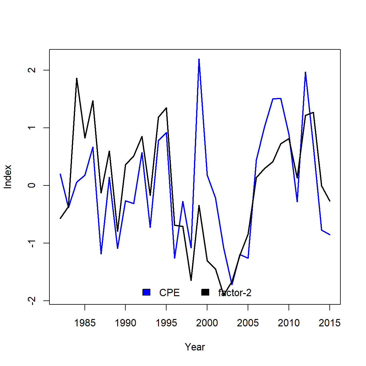
# Plot against cold-pool extent index
index2 = results$Factors$Rotated_loadings$EpsilonTime1[,2]
index2 = sign(cor(index2,CPE)) * index2
png( "EOF_index.png", width=6, height=6, res=200, units="in")
matplot( x=fit$year_labels, y=scale(cbind(CPE,index2)),
type="l", lty="solid", col=c("blue","black"), lwd=2, ylab="Index", xlab="Year" )
legend( "bottom", ncol=2, fill=c("blue","black"), legend=c("CPE","factor-2"), bty="n")
dev.off()
This exercise shows that the cold-pool is associated with an axis that is strongly associated with EOF-2 and to a lesser extent EOF-1
Plotting the optimal rotation of these factors then provides a biological index that is consistent with cold-pool extent in most years:
Caveats
However, as with any multivariate model this model may take a long time (hours-days) to fit. If this is happening please try one or more ways to simplify the problem:
- Use fewer extrapolation-grid cells. With recent versions of VAST, this can be done e.g., using max_cells=1000 for 1000 extrapolation-grid cells.
- Use fewer factors, via decreasing FieldConfig in make_data(.) and/or n_categories in make_settings(.)
- Use fewer knots, via decreasing n_x in make_settings(.)
- Use fewer categories and/or years of data
- Eliminate bias-correction and/or run without getting standard errors.
- Get access to a better computer
- Use MRAN for windows, or other version of R that uses parallelization.
Works cited
Thorson, J. T., Ciannelli, L., & Litzow, M. A. (2020). Defining indices of ecosystem variability using biological samples of fish communities: A generalization of empirical orthogonal functions. Progress in Oceanography, 181, 102244. https://doi.org/10.1016/j.pocean.2019.102244