Seasonal and interannual dynamics
Many regions have monitoring data or opportunistic/process-research collections spanning a wide seasonal window. In these cases, it is helpful to account for both:
- among year variability and
- within year variability in spatial configuration.
In these cases, analysts can use the formula interface to specify covariates that represent the main effect of seasonal and annual variation, and then treat a new ordinal “year-season” variable as t_i within VAST. These main effects for season and year might be linear offsets, spatially varying terms or both, and model selection/exploration is typically needed to determine the best option.
We explore this concept in Thorson et al. 2020, and illustrate a simplified example below. The use of the formula interface for seasonal models was developed by Andrew Allyn. The example starts by formatting the ordinal “year-season” variable, as well as dummy observations to that the model will run for every modeled time:
# load package and example data
library(VAST)
example = load_example( data_set="NWA_yellowtail_seasons" )

# Load data and quick exploration of structure
# Set of years and seasons. The DFO spring survey usually occurs before the NOAA NEFSC spring survey, so ordering accordingly.
year_set = sort(unique(example$sampling_data[,'year']))
season_set = c("DFO", "SPRING", "FALL")

# Create a grid with all unique combinations of seasons and years and then combine these into one "year_season" variable
yearseason_grid = expand.grid("season" = season_set, "year" = year_set)
yearseason_levels = apply(yearseason_grid[,2:1], MARGIN = 1, FUN = paste, collapse = "_")
yearseason_labels = round(yearseason_grid[,'year'] + (as.numeric(factor(yearseason_grid[,'season'], levels = season_set))-1)/length(season_set), digits=1)

# Similar process, but for the observations
yearseason_i = apply(example$sampling_data[,c("year","season")], MARGIN = 1, FUN = paste, collapse = "_")
yearseason_i = factor(yearseason_i, levels = yearseason_levels)

# Add the year_season factor column to our sampling_data data set
example$sampling_data$year_season = yearseason_i
example$sampling_data$season = factor(example$sampling_data$season, levels = season_set)

# Some last processing steps
example$sampling_data = example$sampling_data[, c("year", "season", "year_season", "latitude", "longitude", "swept", "weight")]

# Make dummy observation for each season-year combination
dummy_data = data.frame(
  year = yearseason_grid[,'year'],
  season = yearseason_grid[,'season'],
  year_season = yearseason_levels,
  latitude = mean(example$sampling_data[,'latitude']),
  longitude = mean(example$sampling_data[,'longitude']),
  swept = mean(example$sampling_data[,'swept']),
  weight = 0,
  dummy = TRUE)

# Combine with sampling data
full_data = rbind(cbind(example$sampling_data, dummy = FALSE), dummy_data)

# Create sample data
samp_dat = data.frame(
  "year_season" = as.numeric(full_data$year_season)-1,
  "Lat" = full_data$latitude,
  "Lon" = full_data$longitude,
  "weight" = full_data$weight,
  "Swept" = full_data$swept,
  "Dummy" = full_data$dummy )

# Covariate data. Note here, case sensitive!
cov_dat = data.frame(
  "Year" = as.numeric(full_data$year_season)-1,
  "Year_Cov" = factor(full_data$year, levels = year_set),
  "Season" = full_data$season,
  "Lat" = full_data$latitude,
  "Lon" = full_data$longitude )
# Inspect
table("year_season"=cov_dat$Year, "Actual_year"=cov_dat$Year_Cov)
table("year_season"=cov_dat$Year, "Actual_season"=cov_dat$Season)
After these code-intensive preparatory steps, we build the settings and object, make small modifications to mirror all variance parameters, and then estimate parameters and plot results:
# Make settings
settings = make_settings(n_x = 100,
  Region = example$Region,
  strata.limits = example$strata.limits,
  purpose = "index2",
  FieldConfig = c("Omega1" = 0, "Epsilon1" = 0, "Omega2" = 1, "Epsilon2" = 1),
  RhoConfig = c("Beta1" = 3, "Beta2" = 3, "Epsilon1" = 0, "Epsilon2" = 4),
  ObsModel = c(10, 2),
  bias.correct = FALSE,
  Options = c('treat_nonencounter_as_zero' = TRUE) )

# Creating model formula
formula_use = ~ Season + Year_Cov

# Implement corner constraint for linear effect but not spatially varying effect:
# * one level for each term is 2 (just spatially varying)
# * all other levels for each term is 3 (spatialy varying plus linear effect)
X2config_cp_use = matrix( c(2, rep(3,nlevels(cov_dat$Season)-1), 2, rep(3,nlevels(cov_dat$Year_Cov)-1) ), nrow=1 )

#####
## Model fit -- make sure to use new functions
#####

fit_orig = fit_model("settings" = settings,
  "Lat_i" = samp_dat[, 'Lat'],
  "Lon_i" = samp_dat[, 'Lon'],
  "t_i" = samp_dat[, 'year_season'],
  "b_i" = samp_dat[, 'weight'],
  "a_i" = samp_dat[, 'Swept'],
  #"X1config_cp" = X1config_cp_use,
  "X2config_cp" = X2config_cp_use,
  "covariate_data" = cov_dat,
  #"X1_formula" = ~ 1,
  "X2_formula" = formula_use,
  "X_contrasts" = list(Season = contrasts(cov_dat$Season, contrasts = FALSE), Year_Cov = contrasts(cov_dat$Year_Cov, contrasts = FALSE)),
  "run_model" = FALSE,
  "PredTF_i" = samp_dat[, 'Dummy'] )

# Adjust mapping for log_sigmaXi and fitting final model -- pool variance for all seasons and then set year's to NA
Map_adjust = fit_orig$tmb_list$Map

# Pool variances for each term to a single value
Map_adjust$log_sigmaXi2_cp = factor(c(rep(as.numeric(Map_adjust$log_sigmaXi2_cp[1]), nlevels(cov_dat$Season)),
  rep(as.numeric(Map_adjust$log_sigmaXi2_cp[nlevels(cov_dat$Season)+1]), nlevels(cov_dat$Year_Cov))))

# Fit final model with new mapping
fit  = fit_model("settings" = settings,
  "Lat_i" = samp_dat[, 'Lat'],
  "Lon_i" = samp_dat[, 'Lon'],
  "t_i" = samp_dat[, 'year_season'],
  "b_i" = samp_dat[, 'weight'],
  "a_i" = samp_dat[, 'Swept'],
  #"X1config_cp" = X1config_cp_use,
  "X2config_cp" = X2config_cp_use,
  "covariate_data" = cov_dat,
  #"X1_formula" = formula_use,
  "X2_formula" = formula_use,
  "X_contrasts" = list(Season = contrasts(cov_dat$Season, contrasts = FALSE), Year_Cov = contrasts(cov_dat$Year_Cov, contrasts = FALSE)),
  "newtonsteps" = 0,
  "PredTF_i" = samp_dat[, 'Dummy'],
  "Map" = Map_adjust )

#
out = plot( fit,
  projargs='+proj=natearth +lon_0=-68 +units=km',
  country = "united states of america",
  year_labels = yearseason_labels,
  plot_set = c(3,19),
  mfrow=c(33,3) )
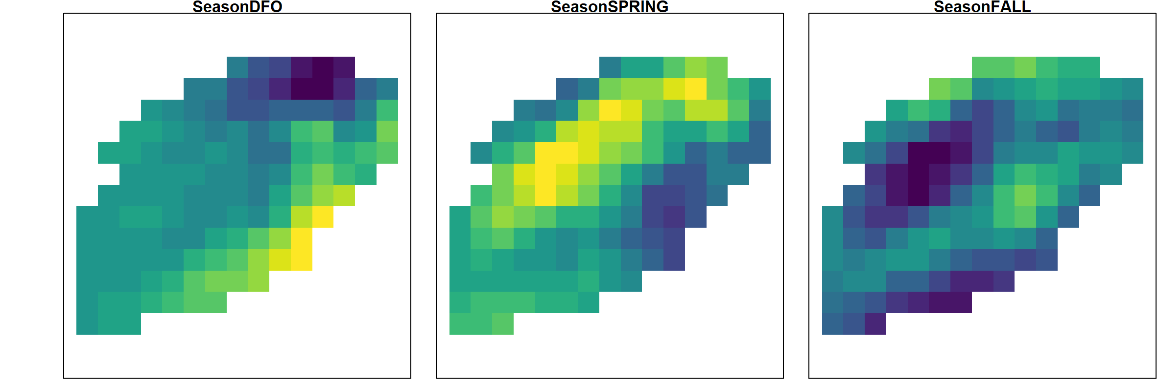
The estimated variance for the annual term goes to zero in this case, so we here visualize the estimated seasonal effects, which shows that the DFO data has higher expected densities along the eastern boundary than the Spring or following Fall NMFS surveys:
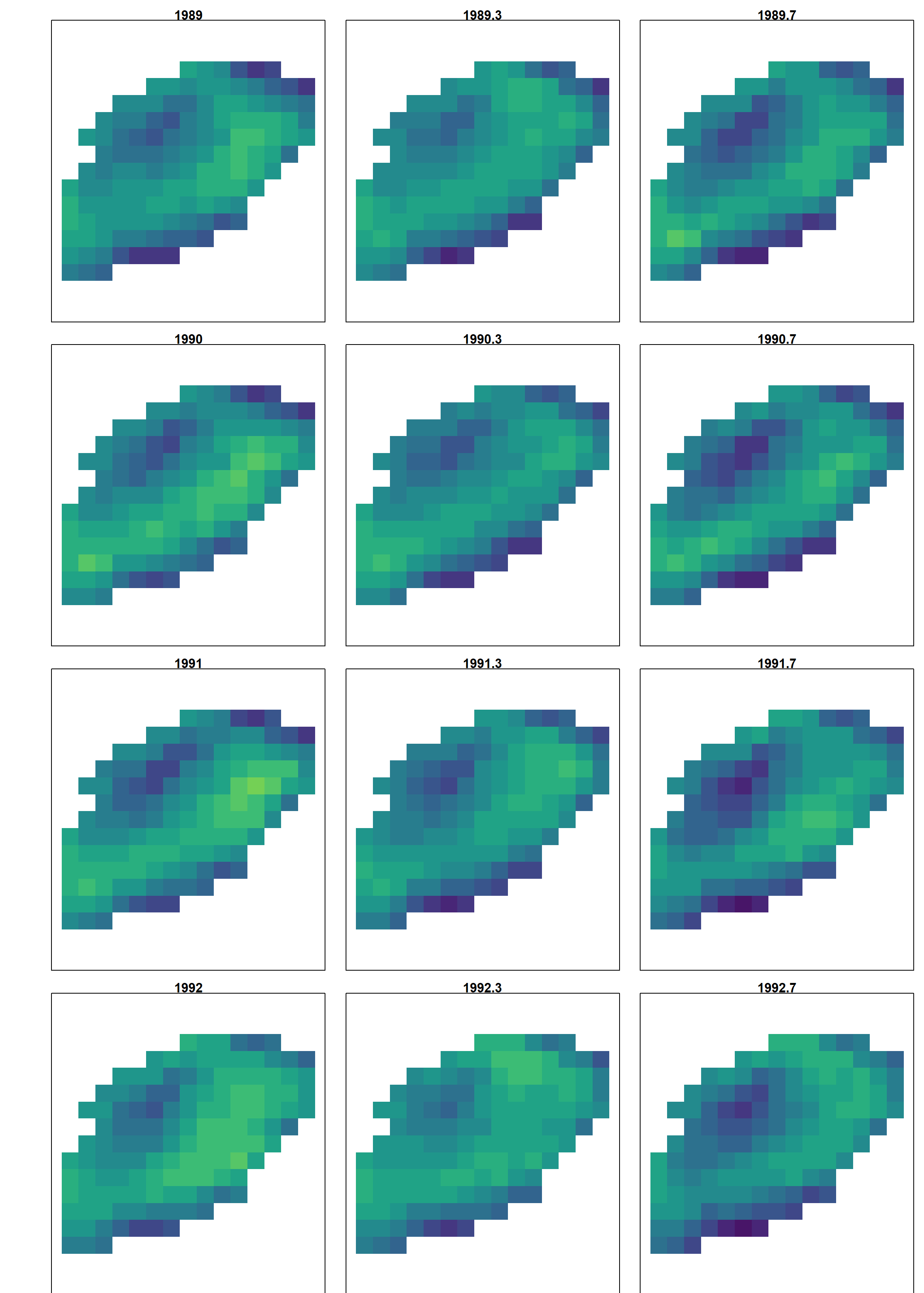
A similar pattern is also apparent in the mapped log-densities for the ordinal year-season variable, which also shows the propagation of hotspots e.g., the southern hotspot from Fall 1989 to DFO 1990 survey intervals:
Works cited
Thorson, J. T., Adams, C. F., Brooks, E. N., Eisner, L. B., Kimmel, D. G., Legault, C. M., Rogers, L. A., et al. 2020. Seasonal and interannual variation in spatio-temporal models for index standardization and phenology studies. ICES Journal of Marine Science, 77: 1879–1892.