Combine data types
Joint models fitting encounter, count, and biomass-sampling data
It is possible to use VAST to fit models jointly to different modes (a.k.a. types) of data, including encounter/non-encounter, count, and biomass-sampling data. Combining data from different sampling designs can be useful to expand the spatial footprint beyond that covered by any one sampling program.
As a simple example, I show code for combining three data types for red snapper in the Gulf of Mexico:
- encounter/non-encounter data from the NMFS Red Snapper/Shark Bottom Longline Survey (“BLL”) dataset;
- count data from the National Marine Fisheries Service (NMFS) Pelagic Acoustic Trawl Survey (“PELACTR”) dataset;
- biomass data from the SEAMAP Groundfish Trawl Survey (“TRAWL”) dataset;
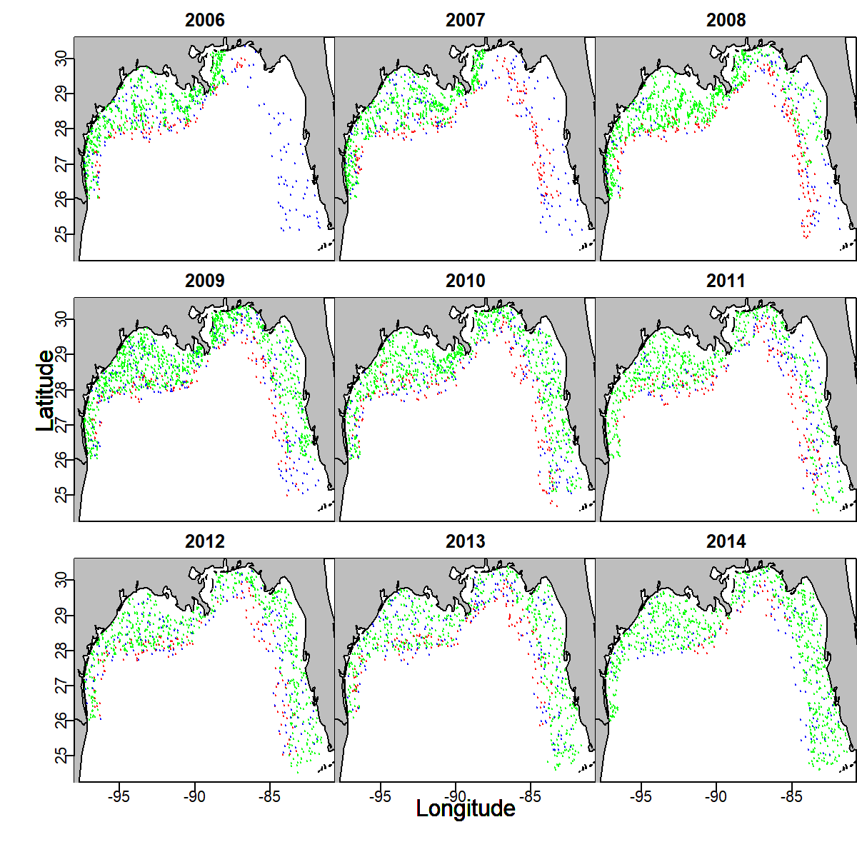
This example is fully documented in Grüss and Thorson (2019). Inspecting the distribution of data (encounter: blue; count: red; biomass: green) shows, e.g.:
- that biomass data are generally lacking in the eastern Gulf of Mexico in 2006-2008, such that other data sources are needed to inform densities and
- that count data are typically hte primary source of information for offshore densities prior to 2014;
In this example, the key change is specifying settings$ObsModel = cbind( c(13,14,2), 1 ). This indicates that observations with:
e_i=0are encounter/non-encounter samples that follow a complementary log-log link from a Poisson point process of numerical density;e_i=1are count-data samples that follow a log-linked Poisson point process of numerical density;e_i=2are biomass samples that follow a Poisson-linked delta model (which approximates a flexible compound-Poisson-gamma distribution), with numerical densities that follow a Poisson point process and a gamma distribution for individual weight;
These three processes then share information about numerical densities (1st linear predictor), while the biomass samples are the only source of information for converting counts to biomass (2nd linear predictor). Importantly, we also include a factor for data type as a catchability coefficient, such that VAST estimates the calibration rate for each gear relative to the reference gear.
# Load packages
library(VAST)

# load data set
# see `?load_example` for list of stocks with example data
# that are installed automatically with `FishStatsUtils`.
example = load_example( data_set="multimodal_red_snapper" )

# Make settings
settings = make_settings( n_x = 100,
  Region = example$Region,
  purpose = "index2",
  strata.limits = example$strata.limits )

# Change `ObsModel` to indicate type of data for level of `e_i`
settings$ObsModel = cbind( c(13,14,2), 1 )

# Add a design matrix representing differences in catchability relative to a reference (biomass-sampling) gear
catchability_data = example$sampling_data[,'Data_type',drop=FALSE]
Q1_formula = ~ factor(Data_type)

# Run model
fit = fit_model( settings = settings,
  Lat_i = example$sampling_data[,'Lat'],
  Lon_i = example$sampling_data[,'Lon'],
  t_i = example$sampling_data[,'Year'],
  c_i = rep(0,nrow(example$sampling_data)),
  b_i = example$sampling_data[,'Response_variable'],
  a_i = example$sampling_data[,'AreaSwept_km2'],
  e_i = as.numeric(example$sampling_data[,'Data_type'])-1,
  Q1_formula = Q1_formula,
  catchability_data = catchability_data )

# Plot results
plot( fit,
      plot_set = c(1,2,3) ) #, col = c("blue","red","green")[catchability_data$Data_type] )
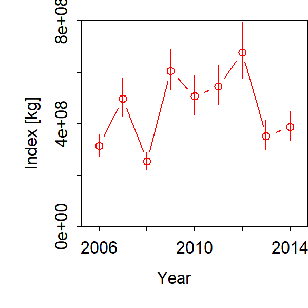
Given these multiple data sets, we can obtain precise estimates of total biomass:
as well as maps of biomass-density:
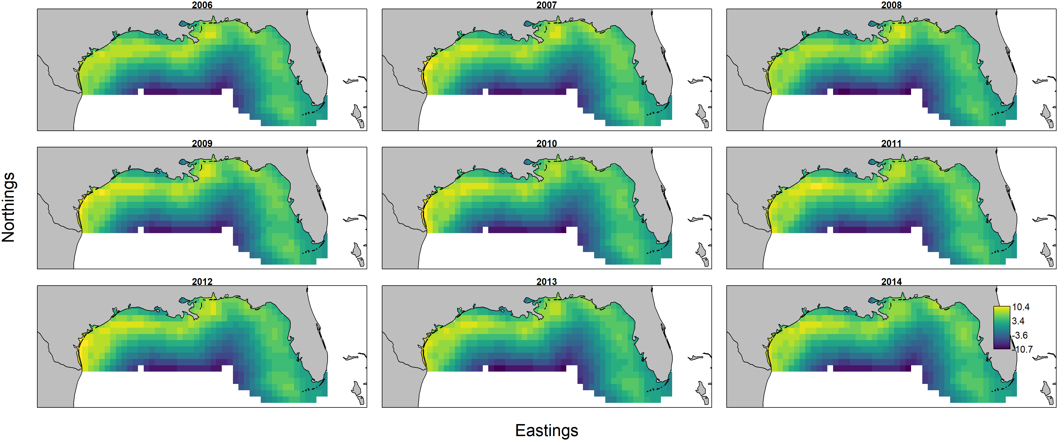
Predicted biomass $d_{s,t} = n_{s,t} w_{s,t}$ is itself the product of predicted numerical density $n_{s,t}$ and individual weight $w_{s,t}$, and these can each be plotted individually by first showing encounter probability:
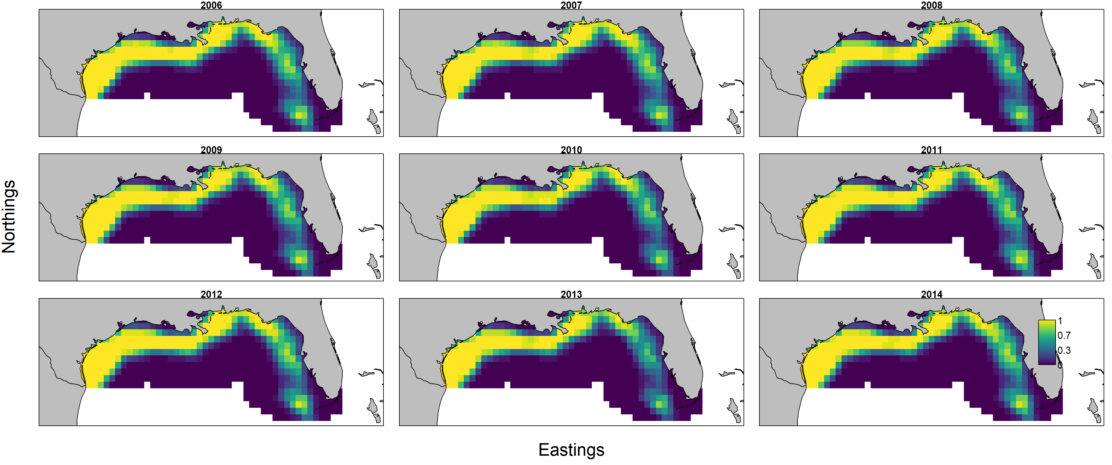
and then showing individual weight:
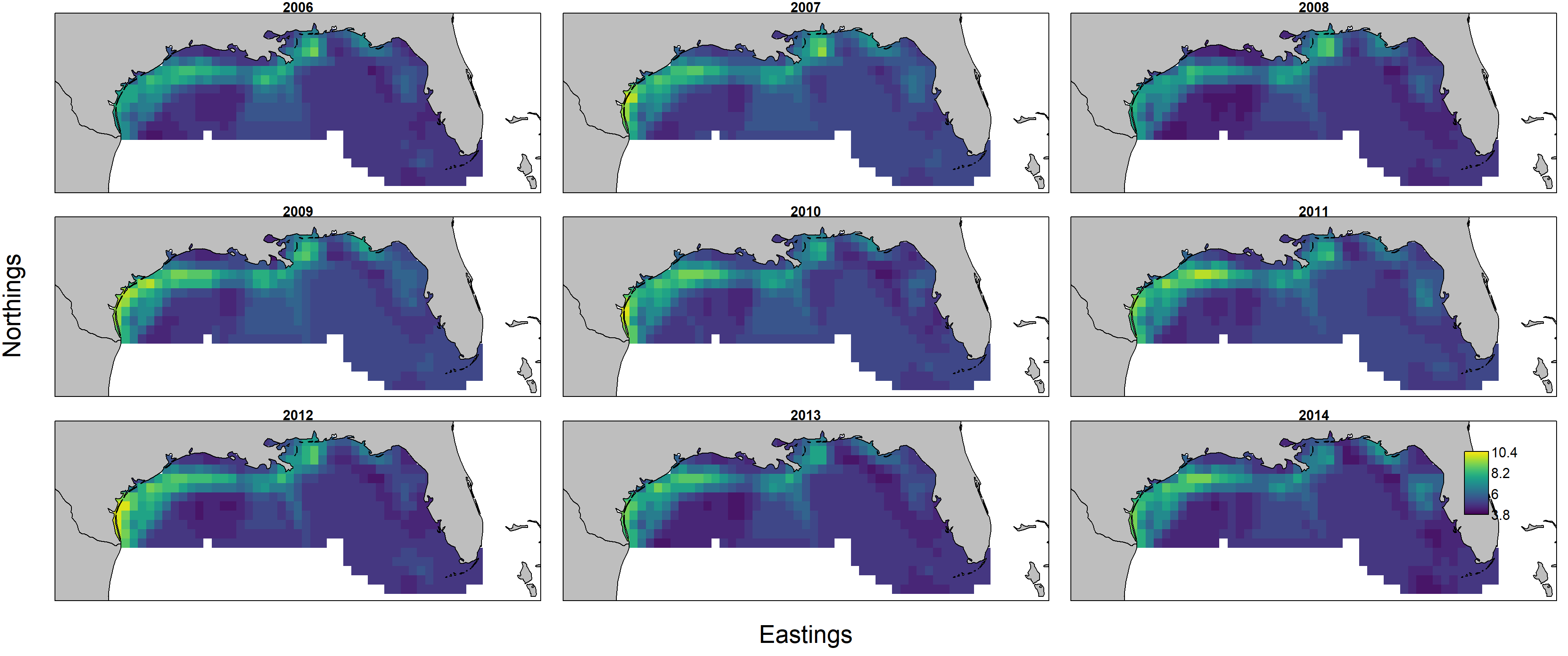
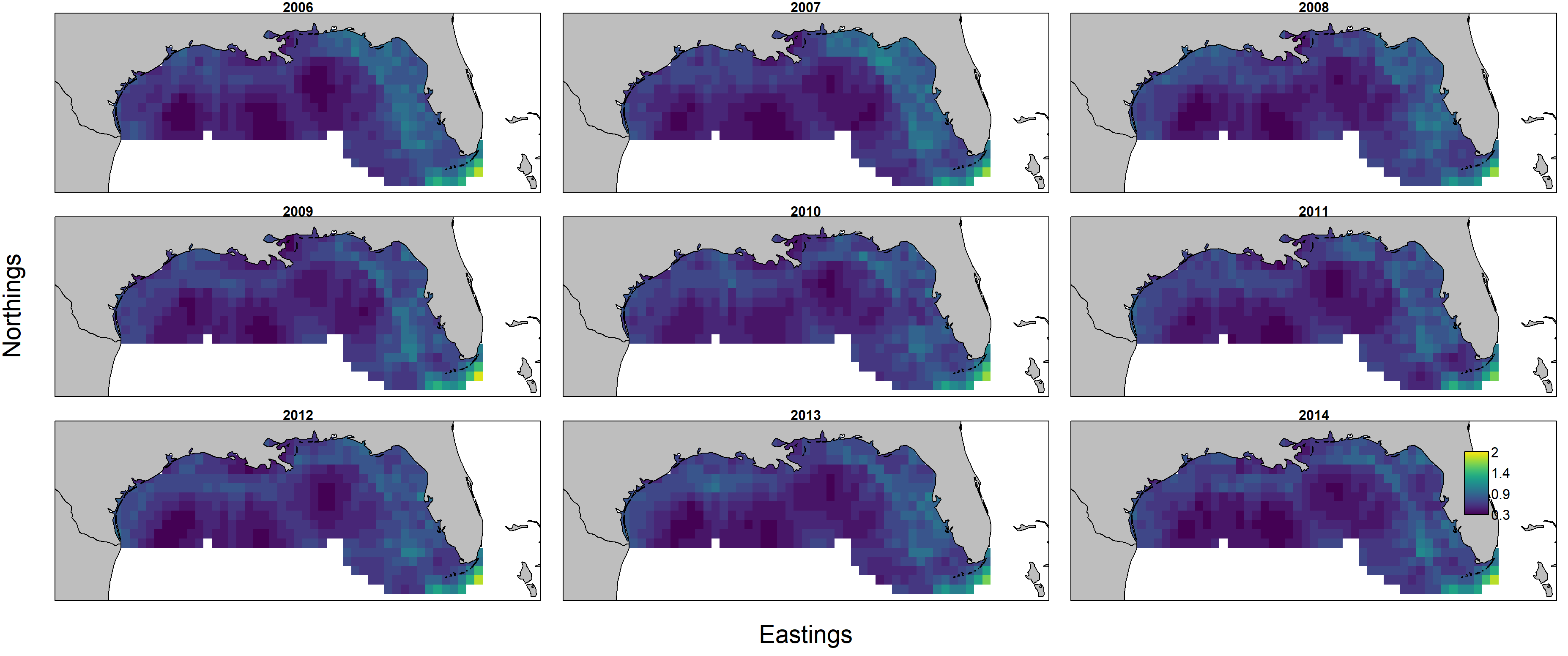
Importantly, encounter probability (resulting from the 1st linear predictor) is informed by all three data sets, but individual weight (resulting from the 2nd linear predictor) is informed only by biomass-sampling data. We can therefore calculate the uncertainty in these two variables:
# Plot SEs
plot( fit,
      plot_set = c(1,2,3),
      plot_value = sd,
      check_residuals = FALSE ) #, col = c("blue","red","green")[catchability_data$Data_type] )
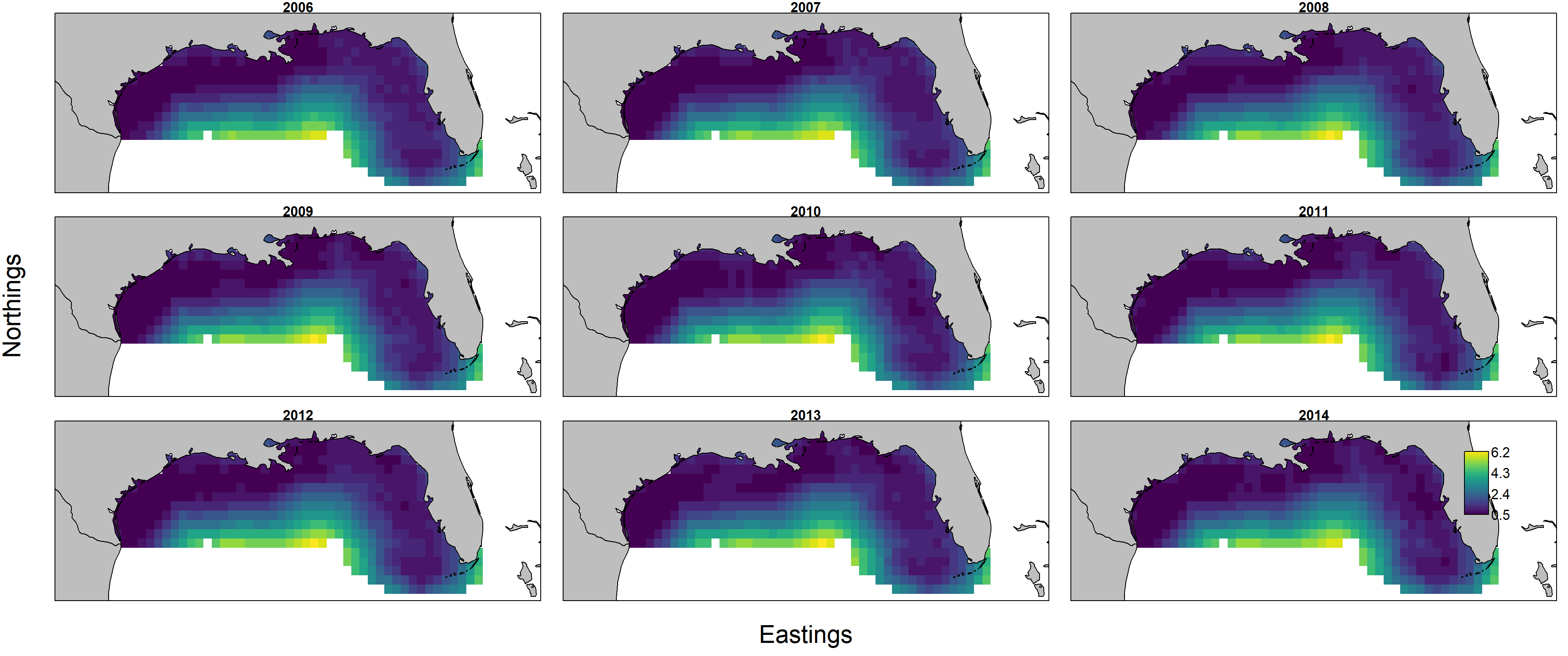
Uncertainty in individual weight then shows higher uncertainty in the eastern Gulf of Mexico in 2006-2007 in particular:
However, a plot of the standard deviation for log-biomass density shows that estimates are relatively imprecise in offshore portions of the modeled domain.
Works cited
Grüss, A., and Thorson, J. T. 2019. Developing spatio-temporal models using multiple data types for evaluating population trends and habitat usage. ICES Journal of Marine Science, 76: 1748–1761.