Correlations between fish condition and density
Joint model for fish condition and density
We developed a multivariate spatio-temporal modeling approach that jointly estimates population density (measured as numbers per area) and fish condition (the relative weight of an individual fish given its body length); the model is then used to predict density-weighted average condition by summing over the product of population density, local condition, and surface area. Density-weighted average condition corrects for biases that would arise when condition (weight-at-length) samples are not distributed proportional to population densities. Our approach treats both density and condition as “categories” in VAST. In models that estimate a covariance between these categories (i.e., using a factor-model for Omega and/or Epsilon), the correlation between the density and condition variables can be interpreted as density dependence (i.e., the causal impact of changing density on changing condition).
This model is based on an allometric equation for weight at length, $W = a L^b$, where $a$ is condition factor and $b$ is allometric scaling of weight-at-length. We then take the log of both sides, $log(W) = log(a) + b * log(L)$, and seek to estimate log-condition factor $log(a)$. To do so, we fit a log-linked spatio-temporal model and include $log(L)$ as a catchability covariate thereby estimating the allometric term $b$ and condition $log(a)$ simultaneously. Here, we demonstrate our approach for the arrowtooth flounder stock in the Gulf of Alaska. The model developed here does not include any environmental covariates, but is simplified from Grüss et al. (2020).
One key step for the estimation of density-dependent fish condition is the definition of the Expansion_cz object. In our case: ` Expansion_cz = matrix( c( 0,0, 2,0 ), ncol = 2, byrow=TRUE )` which specifies that the annual index fish condition will be calculated as the weighted average of local condition, weighted by local densities.
# Load packages
library( VAST )
# load data set
example = load_example( data_set = "GOA_arrowtooth_condition_and_density" )
# Format data
b_i = ifelse( !is.na(example$sampling_data[,'cpue_kg_km2']),
example$sampling_data[,'cpue_kg_km2'],
example$sampling_data[,'weight_g'] )
c_i = ifelse( !is.na(example$sampling_data[,'cpue_kg_km2']), 0, 1 )
catchability_data = data.frame( "log_length_cm" = ifelse(!is.na(example$sampling_data[,'cpue_kg_km2']),
0, log(example$sampling_data[,'length_mm']/10) ))
# Make settings
settings = make_settings( n_x = 250,
Region = example$Region,
purpose = "condition_and_density",
bias.correct = FALSE,
ObsModel = matrix( c(2,4,1,4), ncol=2, byrow=TRUE),
knot_method = "grid" )
settings$FieldConfig[c("Omega","Epsilon"),"Component_1"] = "IID"
Expansion_cz = matrix( c( 0,0, 2,0 ), ncol=2, byrow=TRUE )
settings$ObsModel = matrix( c(2,4, 1,4), ncol=2, byrow=TRUE )
# Run model
fit = fit_model( settings = settings,
Lat_i = example$sampling_data[,'latitude'],
Lon_i = example$sampling_data[,'longitude'],
t_i = example$sampling_data[,'year'],
c_i = c_i,
b_i = b_i,
a_i = rep(1, nrow(example$sampling_data)),
catchability_data = catchability_data,
Q2_formula= ~ log_length_cm,
#Q2config_k = c(3), # Potential switch to make allometric weight-length a spatially varying term
Expansion_cz = Expansion_cz )
# standard plots
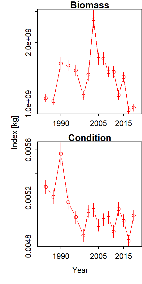
plot( fit,
Yrange=c(NA,NA),
category_names=c("Biomass","Condition (grams per cm^power)") )
Inspecting results, we see that that biomass-weighted condition (weight-at-length in grams per allometric length) has declined for Gulf of Alaska arrowtooth from the 1980s to 2010s. These trends largely differ from the oscillating increase and decrease in total biomass 1990-1996 and again 2003-2009.
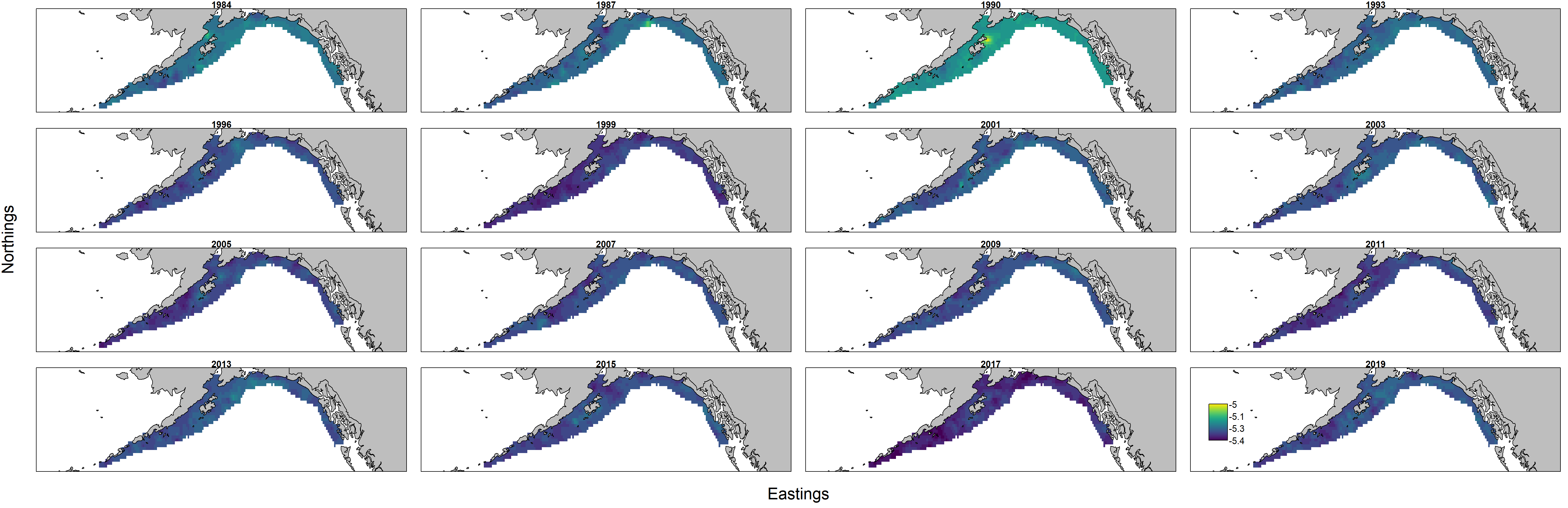
Inspecting maps of log-condition $log(a)$ provides ecological context for these interannual changes. Specifically, we see that log-condition differs more across years (panels) than among locations within a given year.
Alternatively, it is possible to run a similar analysis just on condition (weight and length) data, as shown below. The density maps are unlikely to differ greatly, but this could be useful for comparison with other methods. Of course, only analyzing condition data precludes doing density-weighting when calculating an annual index of condition.
# Load packages
library( VAST )

# load data set
example = load_example( data_set = "GOA_arrowtooth_condition_and_density" )

# Make settings
settings = make_settings( n_x = 250,
  Region = example$Region,
  purpose = "index",
  bias.correct = FALSE,
  knot_method = "grid",
  ObsModel = c(1,4) )

# Only use condition data
condition_data = example$sampling_data
  condition_data = subset( condition_data, is.na(cpue_kg_km2) )

# Run model
fit = fit_model( settings = settings,
  Lat_i = condition_data[,'latitude'],
  Lon_i = condition_data[,'longitude'],
  t_i = condition_data[,'year'],
  b_i = condition_data[,'weight_g'],
  a_i = rep(1, nrow(condition_data)),
  catchability_data = data.frame( "log_length_cm" = log(condition_data[,'length_mm']/10) ),
  #Q2config_k = c(3), # Potential switch to make allometric weight-length a spatially varying term
  Q2_formula= ~ log_length_cm )
Works cited
Grüss, A., Gao, J., Thorson, J.T., Rooper, C., Thompson, G., Boldt, J. and Lauth, R. (2020) Estimating synchronous changes in condition and density in Eastern Bering Sea fishes. Marine Ecology Progress Series.