Ordination

Spatio-temporal ordination

It is possible to use VAST to conduct “ordination.” This process estimates a reduced set of axes that collectively explain variability in a data set. By identifying species that have similar “loadings” for these different axes, ordination can identify species that are similar.

In this example, we use a Tweedie distribution and include temporal variation for each species as fixed effects, while using a saturated covariance in spatial variation, i.e., 5 factors for these five species in the eastern Bering Sea.

# Load packages
library(VAST)

# load data set
example = load_example( data_set="five_species_ordination" )

# Make settings
settings = make_settings( n_x = 50,
  Region = example$Region,
  purpose = "ordination",
  strata.limits = example$strata.limits,
  n_categories = 2,
  ObsModel = c(10,2),
  use_anisotropy = FALSE )

# Eliminate first linear predictor to use Tweedie
# This simplifies interpretation of species assocations by only using one model component
settings$FieldConfig[c('Omega','Epsilon','Beta'),'Component_1'] = c(0,0,'IID')
settings$RhoConfig[c('Beta1','Epsilon1',)] = c(3,0)

# Specify full rank spatial term and eliminate spatio-temporal term
# this makes the demo run faster
settings$FieldConfig[c('Omega','Epsilon','Beta'),'Component_2'] = c(5,0,'IID')
settings$RhoConfig[c('Beta2','Epsilon2')] = c(0,0)

# Run model
fit = fit_model( settings = settings,
  Lat_i = example$sampling_data[,'Lat'],
  Lon_i = example$sampling_data[,'Lon'],
  t_i = example$sampling_data[,'Year'],
  c_i = as.numeric(example$sampling_data[,"species_number"])-1,
  b_i = example$sampling_data[,'Catch_KG'],
  a_i = example$sampling_data[,'AreaSwept_km2'],
  newtonsteps = 0,
  getsd = FALSE,
  test_fit = FALSE,
  category_names = c("pollock", "cod", "arrowtooth", "snow_crab", "yellowfin") )

# Plot results
results = plot( fit,
  plot_set = c(3,17) )

We first inspect the species loadings for spatial variation (omega2) after applying a PCA-rotation by default. This shows that the first three factors collectively explain more than 95% of total explained spatial variation, and subsequent spatial factors could likely be dropped.

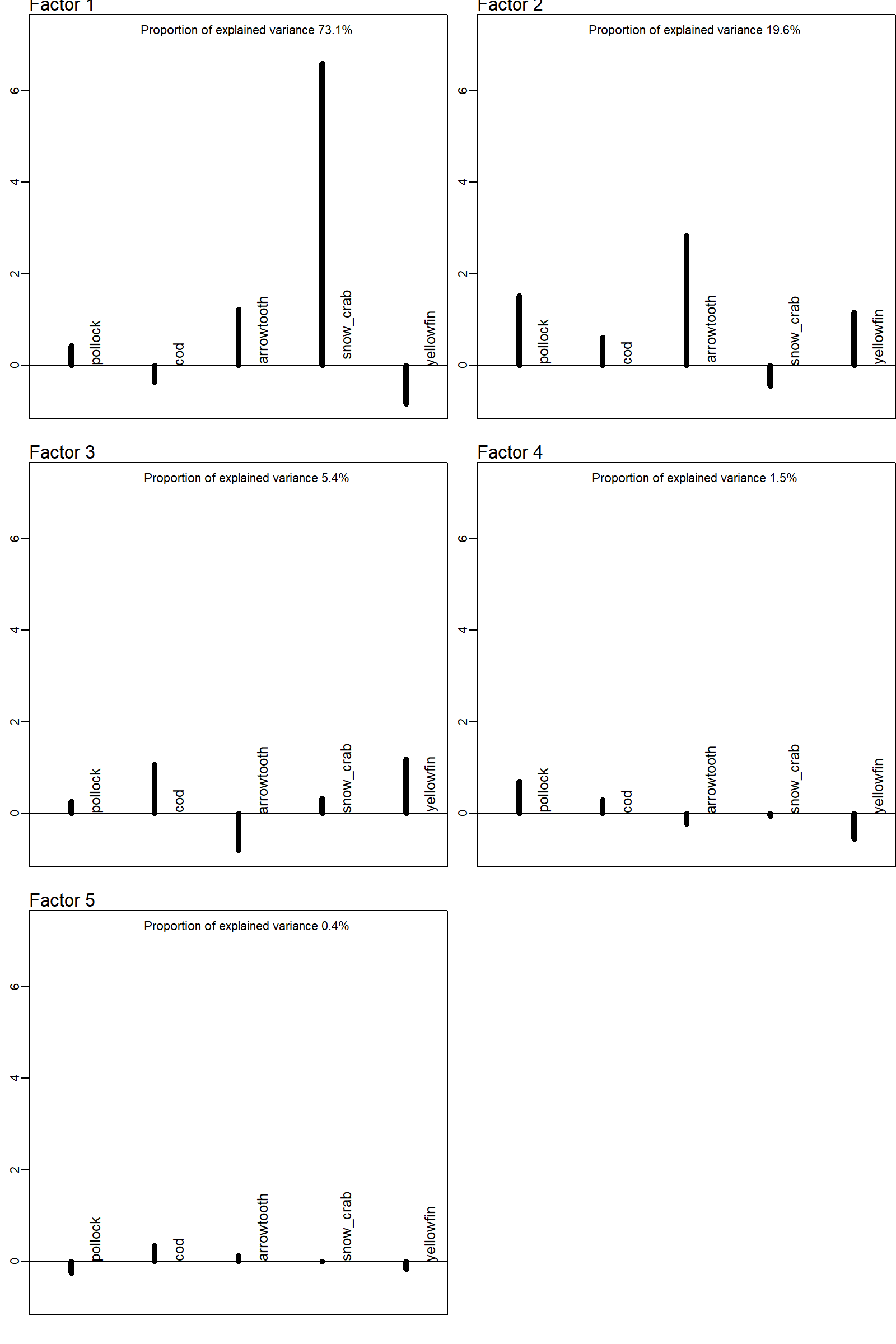
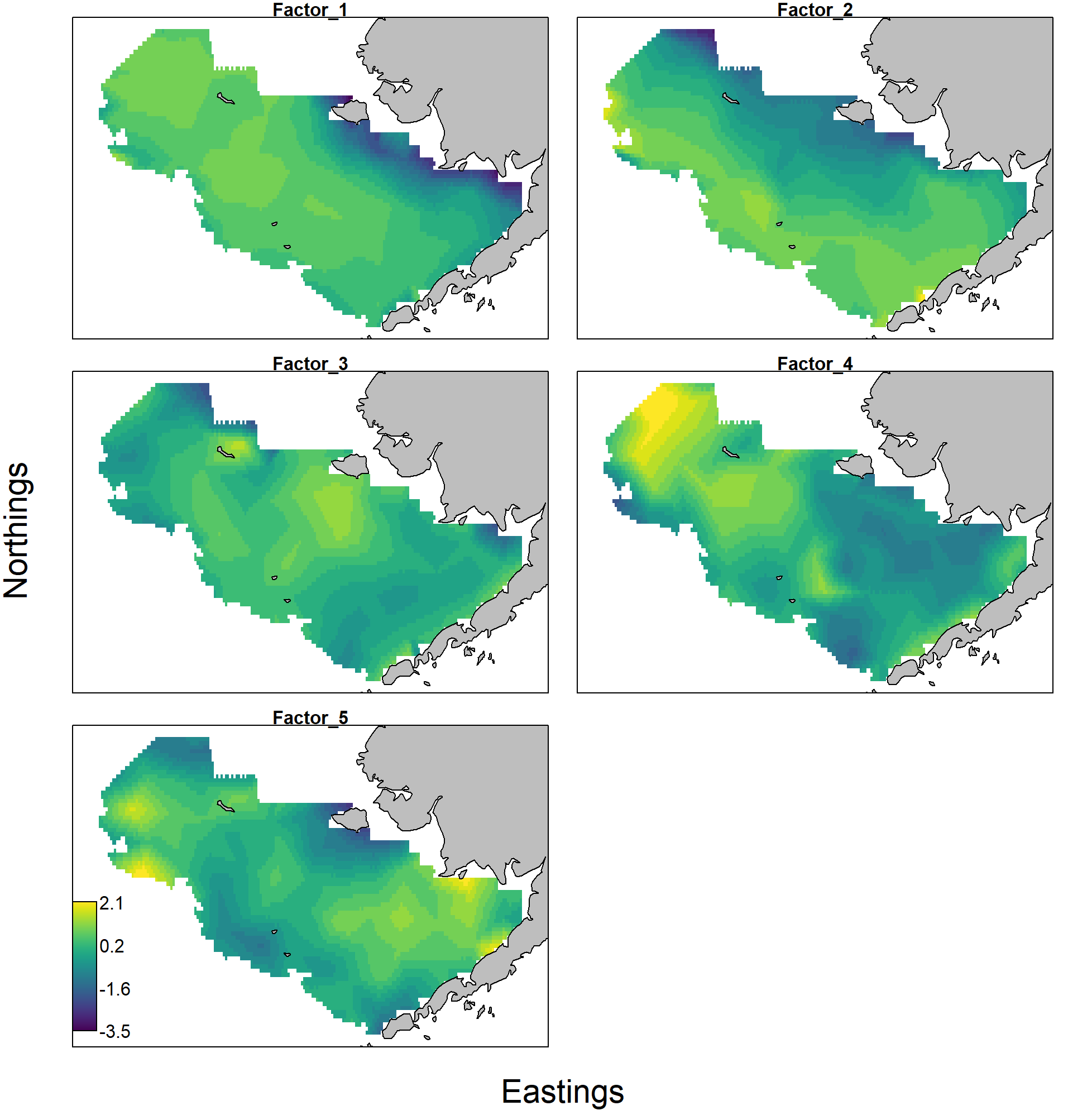
The response maps and factor loadings for these rotated factors show e.g. that:

• the first explains elevated density in the northern portion of the eastern Bering Sea, and is heavily loaded for snow crab, and negative for yellowfin sole and cod;
• the second explains elevated densities along the western portion and into Bristol Bay, and is heavily loaded for pollock and arrowtooth;
• the third (which has minor importance) explains elevated density near Nunivak Island, where cod and yellowfin have relatively higher density than arrowtooth;

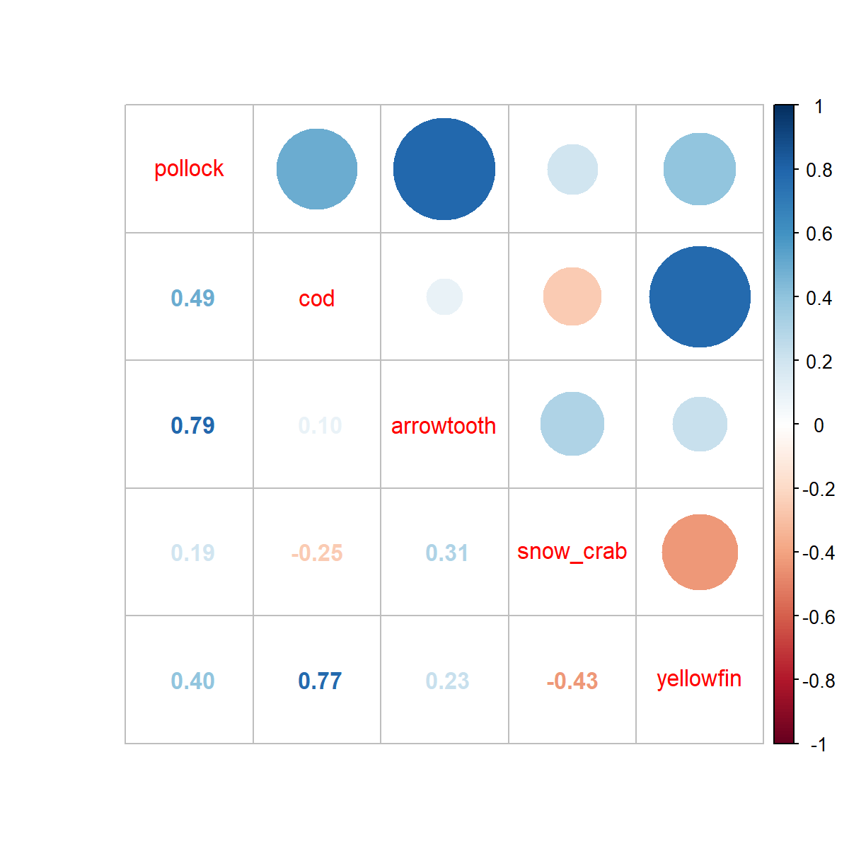
We can also plot the covariance in spatial variation (omega2) that arises from these factors. This then shows that snow crab has relatively little correlation with any other species, while pollock and arrowtooth are highly correlated, and similarly yellowfin and cod.

# Plot correlations (showing Omega1 as example)
require(corrplot)
png( "correlations.png", width=6, height=6, res=200, units="in")
  Cov_omega2 = fit$Report$L_omega2_cf %*% t(fit$Report$L_omega2_cf)
  corrplot( cov2cor(Cov_omega2), method="pie", type="lower")
  corrplot.mixed( cov2cor(Cov_omega2) )
dev.off()

Works cited

Thorson, Scheuerell, M. D., Shelton, A. O., See, K. E., Skaug, H. J., and Kristensen, K. 2015. Spatial factor analysis: a new tool for estimating joint species distributions and correlations in species range. Methods in Ecology and Evolution, 6: 627-637.