Joint model of stomach contents and density
Joint model for stomach content, predator biomass catch rate, and predator-expanded-stomach-contents (PESCs)
We developed an approach that fits a spatio-temporal model with VAST to both prey-biomass-per-predator-mass data (i.e., the ratio of prey biomass in stomachs to predator weight) and predator biomass catch rate data (predator biomass per unit area), to predict “predator-expanded-stomach-contents” (PESC; the product of prey-biomass-per-predator-biomass, predator biomass per unit area, and surface area). The PESC estimates can be used to visualize either the annual landscape of PESC (spatio-temporal variation), or can be aggregated across space to calculate annual variation in diet proportions (variation among prey items and among years).
Here, we demonstrate our approach in a data-limited situation involving West Florida Shelf red grouper (Epinephelus morio, Epinephelidae) for 2011-2015. Four prey items are considered: crabs, fish, shrimps, and “other prey”. We demonstrate how diet proportions are calculated from the PESCs estimated by our model.
One key step for the estimation of PESCs is the definition of the Expansion_cz object. In our case:
Expansion_cz = matrix( c( 0, 0, 1, 0, 1, 0, 1, 0, 1, 0 ), nrow = nlevels( sampling_data[,"spp"] ), ncol = 2, byrow = TRUE )
which entails that the estimated biomass (the product of biomass per unit area and surface area) for the first “category”, namely the predator (red grouper), will be multiplied by the estimated prey-biomass-per-predator-biomass for the other categories, namely the prey items (crabs, fish, other prey, and shrimps), to obtain PESC estimates (for crabs, fish, other prey, and shrimps).
For more information about the approach and its outcomes, please read Gruss et al. (2020). As case study we analyze red group biomass as predator, combined with their consumption of fishes, crabs, shrimps, or other prey. We start by illustrating how to format separate data sets containing predator density and stomach samples into a single data frame:
# Load packages
library( VAST )

# We load two datasets:
# (1) A predator biomass catch rate dataset, where biomass catch rate is in kg per square-km
# (2) A stomach content dataset, providing prey biomass data (in g) and predator mass data (in g)
example = load_example( data_set = "PESC_example_red_grouper" )

# Modify the predator biomass catch rate dataset. Specifically:
# (1) Assign a new "Category" field to the dataset (with the unique level "Red_grouper")
example$Predator_biomass_cath_rate_data$Category = as.factor( "Red_grouper" )
# (2) Rename the "CPUE_kg_km2" field into "Response_variable" - to allow for
# the merging of the predator biomass catch rate and stomach content datasets
names( example$Predator_biomass_cath_rate_data )[4] <- "Response_variable"
# Note that a_i = 1 because `Response_variable` is already KG per KM^2; Future
# applications could instead treate `Response_variable` as KG and use `a_i` as
# area swept

# Modify the stomach content dataset. Specifically:
# (1) Create a new "predator-biomass-per-predator-mass" variable (in g per g of predator), by dividing
# prey biomass (in g) by predator mass (in g)
example$Stomach_content_data$Prey_biomass_per_predator_mass <- example$Stomach_content_data$Prey_biomass_in_stomach_g /
	example$Stomach_content_data$Predator_mass_g
# (2) Rename the "Prey_item" field into "Category" (levels: "Crabs", "Fish", "Shrimps", and "Other") - to allow for
# the merging of the predator biomass catch rate and stomach content datasets
example$Stomach_content_data$Category <- as.factor( example$Stomach_content_data$Prey_item )
# (3) Reorder the columns of the dataset - to allow for
# the merging of the predator biomass catch rate and stomach content datasets
example$Stomach_content_data <- example$Stomach_content_data[,c( 1 : 3, 8, 7, 9 )]
# (4) Rename the "predator-biomass-per-predator-mass" field into "Response_variable" - to allow for
# the merging of the predator biomass catch rate and stomach content datasets
names( example$Stomach_content_data )[4] <- "Response_variable"
# (5) Change a_i = 1, because `Response_variable` is already prey-G per predator-G, such that
# product of c=0 and c = {1,2,3,4} has units KG
example$Stomach_content_data$Area_swept_km2 = 1
# Note that future applications could instead treat
# `Response_variable` as prey-biomass and `a_i` as predator-body-size

# Merge the predator biomass catch rate and stomach content datasets
sampling_data <- rbind( example$Predator_biomass_cath_rate_data, example$Stomach_content_data )
After these preparatory steps, we proceed with fitting VAST and plotting output using the normal steps:
# Make settings
settings = make_settings( n_x = 300,
  Region = example$Region,
  purpose = "index2",
  strata.limits = example$strata.limits,
  use_anisotropy = FALSE,
  fine_scale = FALSE,
  bias.correct = FALSE )

# Set up the "Expansion_cz" input
# We want the estimated biomass (the product of biomass per unit area and surface area)
# for the first “category”, namely the predator (red grouper) to be multiplied by
# the estimated prey-biomass-per-predator-biomass for the other categories, namely the prey items
# (crabs, fish, other prey, and shrimps), to obtain PESC estimates (for crabs, fish, other prey, and shrimps).
Expansion_cz = matrix( byrow = TRUE,
  nrow = nlevels( sampling_data[,"Category"] ),
  ncol = 2,
  data = c( 0, 0,
            1, 0,
            1, 0,
            1, 0,
            1, 0 ) )

# Run the model
fit = fit_model( settings = settings,
    Lat_i = sampling_data[,'Lat'],
    Lon_i = sampling_data[,'Lon'],
    t_i = as.numeric( sampling_data[,'Year'] ),
    c_i = as.numeric( sampling_data[,'Category'] ) - 1,
    b_i = sampling_data[,'Response_variable'],
    a_i = sampling_data[,'Area_swept_km2'],
    Expansion_cz = Expansion_cz,
    input_grid = example$input_grid,
    Npool = 20,
    getsd = TRUE,
    test_fit = FALSE,
    category_names = levels(as.factor(sampling_data[,'Category'])) )

# Calculate and plot diet proportions
plots = plot( fit,
              year_labels = 2011:2015 )
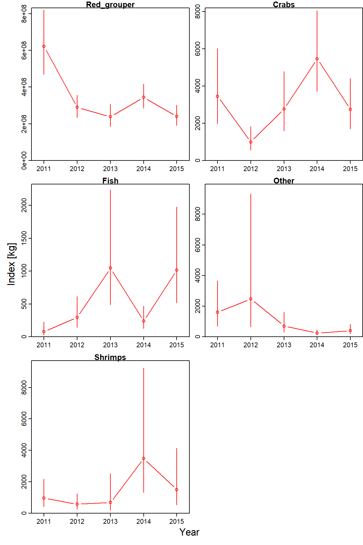
Indices of predator biomass and predator-expanded stomach contents shows that predator biomass has decreased, but that per-biomass consumption has increased factor resulting in a net increase in predicted predator-expanded stomach contents for fishes and crabs.
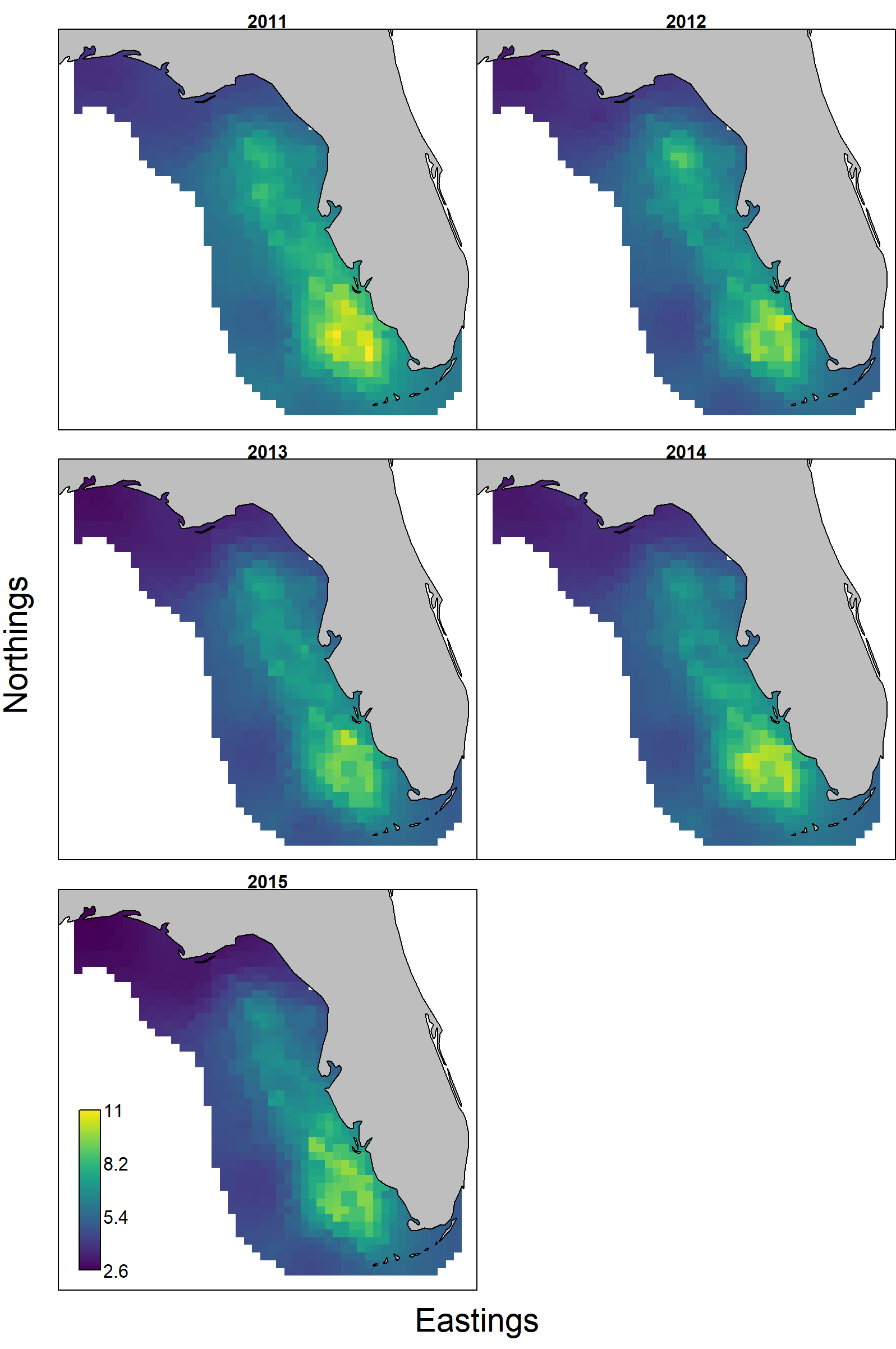
To better interpret these patterns, we first inspect the predator biomass landscale and see that red grouper consistently has highest density in the southern portion of our spatial domain, but densities in the northern portion have declined faster than the south.
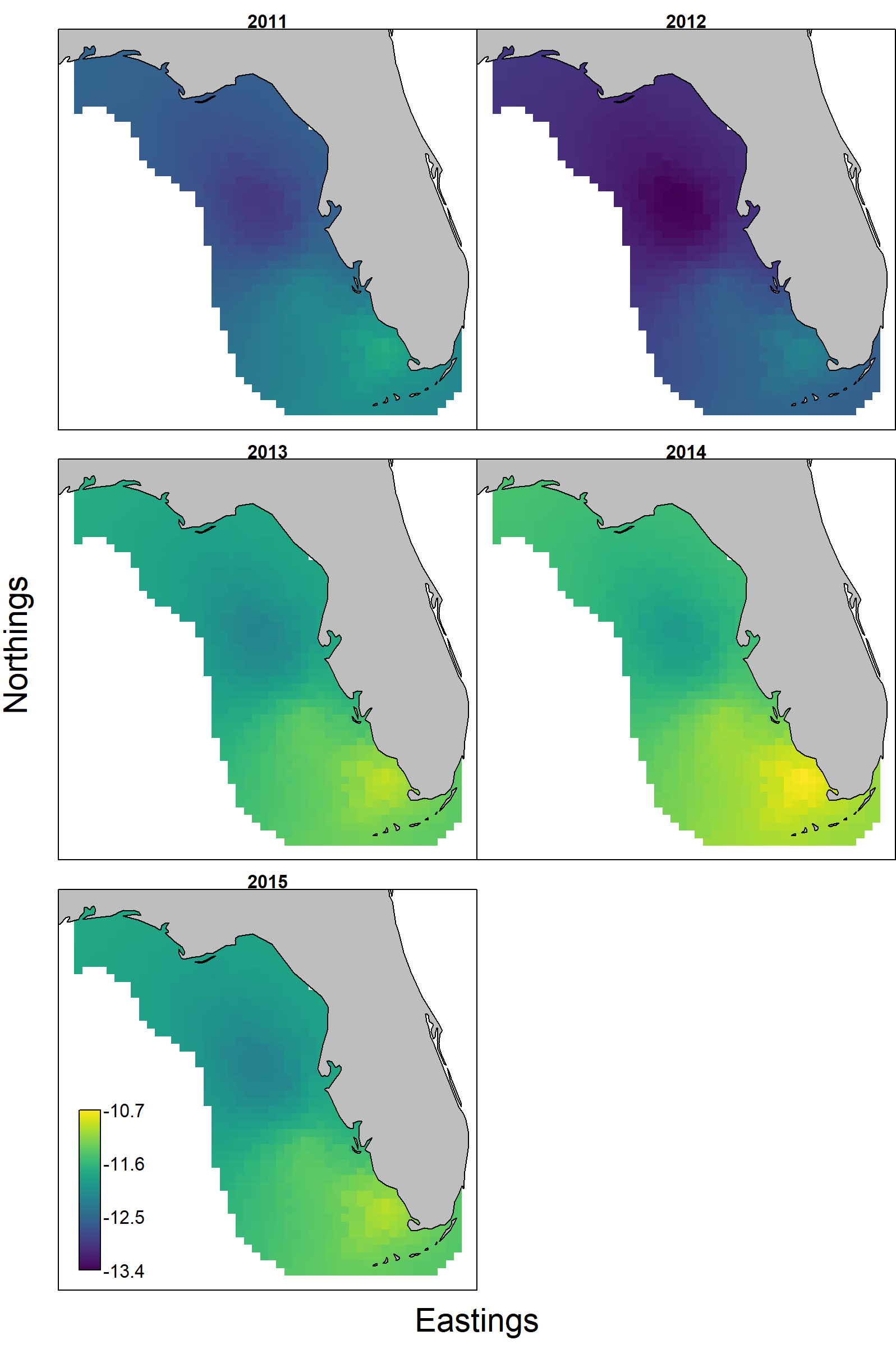
Finally, (and using crab as single example) the per-biomass consumption of crabs is higher near the Florida keys and low in the northern portion of red grouper distribution. This per-biomass consumption has rapidly increased from 2011-2015 with proportional increases throughout the spatial domain.
Works cited
Grüss A, Thorson JT, Carroll G, Ng EL, Holsman KK, Aydin K, Kotwicki S, Morzaria-Luna HM, Ainsworth CH, Thompson KA (2020). Spatio-temporal analyses of marine predator diets from data-rich and data-limited systems. Fish and Fisheries, 21: 718-739.