EcoState as surplus production model

library(ecostate)
library(JABBA)
library(spict)
set.seed(101)

ecostate is an R package for fitting the mass-balance dynamics specified by EcoSim as a state-space model. It can be used as a surplus production model by treating a single species as a “producer”

Simulation demonstration

We first simulate new data. To do so, we simulate a Schaefer production model with Gompertz effort dynamics:

# Time-interval
years = 1981:2020
n_years = length(years)

# Biology
r = 0.2
#MSY = 100
K = 1000
sigmaB = 0.5
B0 = K * exp(sigmaB*rnorm(1))
prod_func = c("Schaefer", "Fox")[2]

# Effort dynamics
Bequil = 0.4 * K
Brate = 0.2
sigmaE = 0.1
E0 = 0.01

# Survey
q = 1
sigmaQ = 0.1

#
Pbar_t = P_t = C_t = E_t = B_t = rep(NA, n_years)
B_t[1] = B0
E_t[1] = E0

#
for( t in 2:n_years ){
  if(prod_func=="Scaefer") Pbar_t[t] = B_t[t-1] + r * B_t[t-1] * (1 - B_t[t-1]/K)
  if(prod_func=="Fox") Pbar_t[t] = r * B_t[t-1] * log(K / B_t[t-1])
  P_t[t] = Pbar_t[t] * exp(sigmaB*rnorm(1))
  B_t[t] = B_t[t-1] + P_t[t]
  E_t[t] = E_t[t-1] * (B_t[t-1]/Bequil)^Brate * exp(sigmaE*rnorm(1))
  C_t[t] = B_t[t] * (1 - exp(-E_t[t]))
  B_t[t] = B_t[t] - C_t[t]
}
Bobs_t = q * B_t * exp(sigmaQ * rnorm(n_years))

# 
matplot( x=years, y=cbind(B_t,Bobs_t,C_t), type="l", log="y", lty="solid")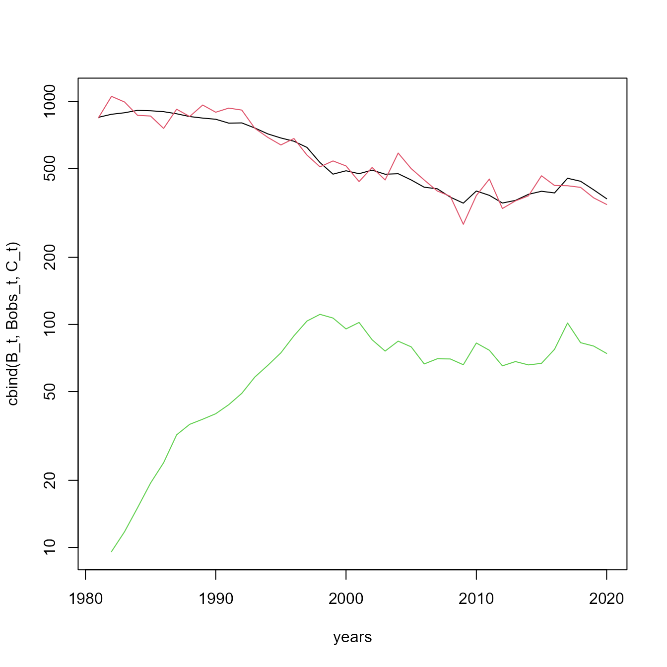

We then set up inputs to EcoState

# Name taxa (optional, for illustration)
taxa = "target"
n_taxa = length(taxa)

# Ecopath-with-EcoSim parameters
# Diet matrix
DC_ij = array( 0, dim=c(1,1) )
PB_i = 0.1
QB_i = NA
EE_i = 1
B_i = 1
U_i = 0.2
type_i = "auto"
X_ij = array( 2, dim=c(1,1) )

# reformat to longform data-frame
Catch = na.omit(data.frame( "Mass" = C_t, "Year" = years, "Taxon" = taxa ))
Biomass = data.frame( "Mass" = Bobs_t, "Year" = years, "Taxon" = taxa )

Next, we fit them with ecostate

# Settings: specify what parameters to estimate
fit_eps = taxa   # process errors
fit_Q = taxa       # catchability coefficient
fit_B0 = c()      # non-equilibrium initial condition
fit_B = taxa       # equilibrium biomass
fit_PB = taxa     # Productivity _propto_ natural mortality

# Treat it as an autotroph (given there's no prey to consume)
type = "auto"

# Label EwE inputs for each taxon as expected (so users can easily change taxa)
names(PB_i) = names(QB_i) = names(B_i) = names(EE_i) = names(type) = names(U_i) = taxa
  dimnames(DC_ij) = dimnames(X_ij) = list("Prey"=taxa, "Predator"=taxa)
  
# Define priors
log_prior = function(p){
  # Prior on productivity
  logp = dnorm( p$logPB_i, mean=log(0.1), sd=0.5, log=TRUE )
  # Prior on process-error log-SD to stabilize model
  logp = logp + dnorm( p$logtau_i, mean=log(0.2), sd=1, log=TRUE )
  # Prior on vulnerability to stabilize model
  logp = logp + dnorm( p$Xprime_ij[1,1], mean=0, sd=1, log=TRUE )
}

# Run model
out0 = ecostate( taxa = taxa,
                years = years,
                catch = Catch,
                biomass = Biomass,
                PB = PB_i,
                QB = QB_i,
                DC = DC_ij,
                B = B_i,
                EE = EE_i,
                X = X_ij,
                type = type,
                U = U_i,
                fit_B = fit_B,
                fit_Q = fit_Q,
                fit_eps = fit_eps,
                fit_B0 = fit_B0,
                fit_PB = fit_PB,
                log_prior = log_prior,
                control = ecostate_control( nlminb_loops = 0,
                                            getsd = FALSE,
                                            start_tau = 0.1 ) )

# Estimate logPB
pars = out0$tmb_inputs$p
map = out0$tmb_inputs$map
map$Xprime_ij = factor(1)

# Run model
out = ecostate( taxa = taxa,
                years = years,
                catch = Catch,
                biomass = Biomass,
                PB = PB_i,
                QB = QB_i,
                DC = DC_ij,
                B = B_i,
                EE = EE_i,
                X = X_ij,
                type = type,
                U = U_i,
                fit_B = fit_B,
                fit_Q = fit_Q,
                fit_eps = fit_eps,
                fit_B0 = fit_B0,
                fit_PB = fit_PB,
                log_prior = log_prior,
                control = ecostate_control( map = map,
                                            tmb_par = pars ) )
#> Using `control$tmb_par`, so be cautious in constructing it
#> Using `control$map`, so be cautious in constructing it

# print output to terminal
out
#> Dynamics integrated using  ABM  with  10  time-steps
#> Run time: Time difference of 4.512951 secs
#> Negative log-likelihood: -74.51341
#> 
#> EcoSim parameters:
#>        type QB        PB        B EE   U
#> target auto NA 0.1588959 1357.543  0 0.2
#> 
#> EcoSim diet matrix:
#>         Predator
#> Prey     target
#>   target      0
#> 
#> EcoSim vulnerability matrix:
#>         Predator
#> Prey       target
#>   target 1.357989
#> 
#> Estimates: sdreport(.) result
#>             Estimate Std. Error
#> logB_i     7.2134320  0.3091545
#> logPB_i   -1.8395058  0.4064990
#> Xprime_ij -1.0272522  0.6851844
#> logtau_i  -3.0608084  0.4094129
#> logq_i    -0.3785607  0.3285576
#> Maximum gradient component: 0.000126564

Finally we can calculate a function that calculates the annualized surplus production

# Define function to calculate annualized production
prod_fun = function( biomass, Xprime, logPB, taxon, ecofit ){
  p = ecofit$internal$parhat
  n_taxa = length(ecofit$internal$taxa)
  if(!missing(Xprime)) p$Xprime_ij[] = Xprime
  if(!missing(logPB)) p$logPB_i[] = logPB
  if(missing(taxon)) taxon = ecofit$internal$taxa[n_taxa]
  p = add_equilibrium( p,
                       scale_solver = ecofit$internal$control$scale_solver,
                       noB_i = ifelse(is.na(p$logB_i),1,0),
                       type_i = type_i )
  p$logF_i = rep(log(0), n_taxa)
  p$epsilon_i = rep(0, n_taxa)
  p$nu_i = rep(0, n_taxa)
  p$phi_g2 = rep(0, ecofit$internal$settings$n_g2)
  State = c( ecofit$rep$out_initial$B_i, rep(0,n_taxa) )
  State[match(taxon,ecofit$internal$taxa)] = biomass
  #dBdt(Time=0, State=State, Pars=p)
  proj = abm3pc_sys(
        f = dBdt,
        a = 0, 
        b = 1,
        n = ecofit$internal$control$n_steps,
        Pars = p,
        type_i = type_i,
        n_species = n_taxa,
        F_type = "integrated",
        y0 = State )
  biomass1 = rev( proj$y[,match(taxon,ecofit$internal$taxa)] )[1]
  return( biomass1 - biomass )
}

We then use that function to compare the exact and an approximation that uses a first-order Euler approximation:

# Calculate predicted and true curves
x = seq(0, 2*K, length=1000)[-1]
if(prod_func=="Scaefer") y = r * x * (1 - x/K)
if(prod_func=="Fox") y = r * x * log(K/x)
yhat = sapply( x, FUN=prod_fun, ecofit=out,
               Xprime = out$internal$parhat$Xprime_ij, 
               logPB = out$internal$parhat$logPB_i )

# Solve for Bmsy / B0 in production function
dBdt_approx = function(b, x, p){
  # dBdt for single autotroph (not annualized)
  dBdt_expr = expression(b * p * (1-b) / (x - 1 + b))
  # Solve for d/db dBdt = 0 as min_b((d/db dBdt)^2)
  #eval( D(dBdt,"b") )^2
  # OR:  -dBdt
  eval(dBdt_expr)
}
phi1 = optimize( dBdt_approx, lower=0.01, upper=0.99, maximum=TRUE,
                x = 1+exp(out$internal$parhat[['Xprime_ij']][1,1]), 
                p = exp(out$internal$parhat[['logPB_i']]) )$maximum
# Empirical
phi2 = x[which.max(yhat)] / 1000 
#
msy1 = exp(out$internal$parhat$logB_i) * dBdt_approx(phi1, 
                x = 1+exp(out$internal$parhat[['Xprime_ij']][1,1]), 
                p = exp(out$internal$parhat[['logPB_i']]) )
#
msy2 = yhat[which.max(yhat)]
# 
true_msy = y[which.max(y)]

# Plot them
plot( x=x, y=y, type="l", xlim=c(0,2*K), ylim=c(0,2*max(y)), lwd=3, 
      xlab="Biomass", ylab="Annual surplus production" )
lines( x=x, y=yhat, lwd=3, col="red" )    # *exp(out$internal$parhat$logq_i)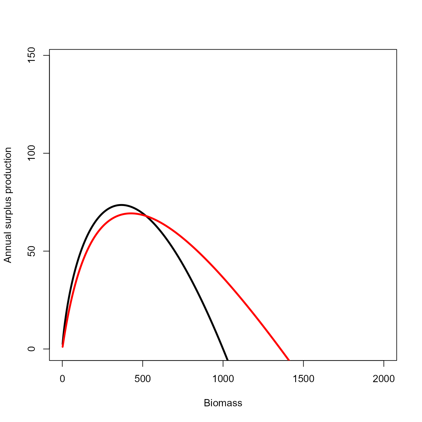

And we can also plot the estimated and true biomass

# Extract estimated biomass
Bhat_t = out$derived$Est$B_ti
Bse_t = out$derived$SE$B_ti

# Reformat to long-form data frame for ggplot
results = cbind( "Year" = years,
                 "True" = as.vector(B_t),
                 "Obs" = as.vector(Bobs_t),
                 "Est" = as.vector(Bhat_t),
                 "SE" = as.vector(Bse_t) )

# Plot using ggplot
library(ggplot2)
ggplot(results) + 
  geom_line( aes(x=as.numeric(Year), y=True), colour="red" ) + 
  geom_line( aes(x=as.numeric(Year), y=Obs) ) + 
  geom_line( aes(x=as.numeric(Year), y=Est), linetype="dotted" ) +
  geom_ribbon( aes(x=as.numeric(Year), ymin=Est-1.96*SE, ymax=Est+1.96*SE), alpha=0.2)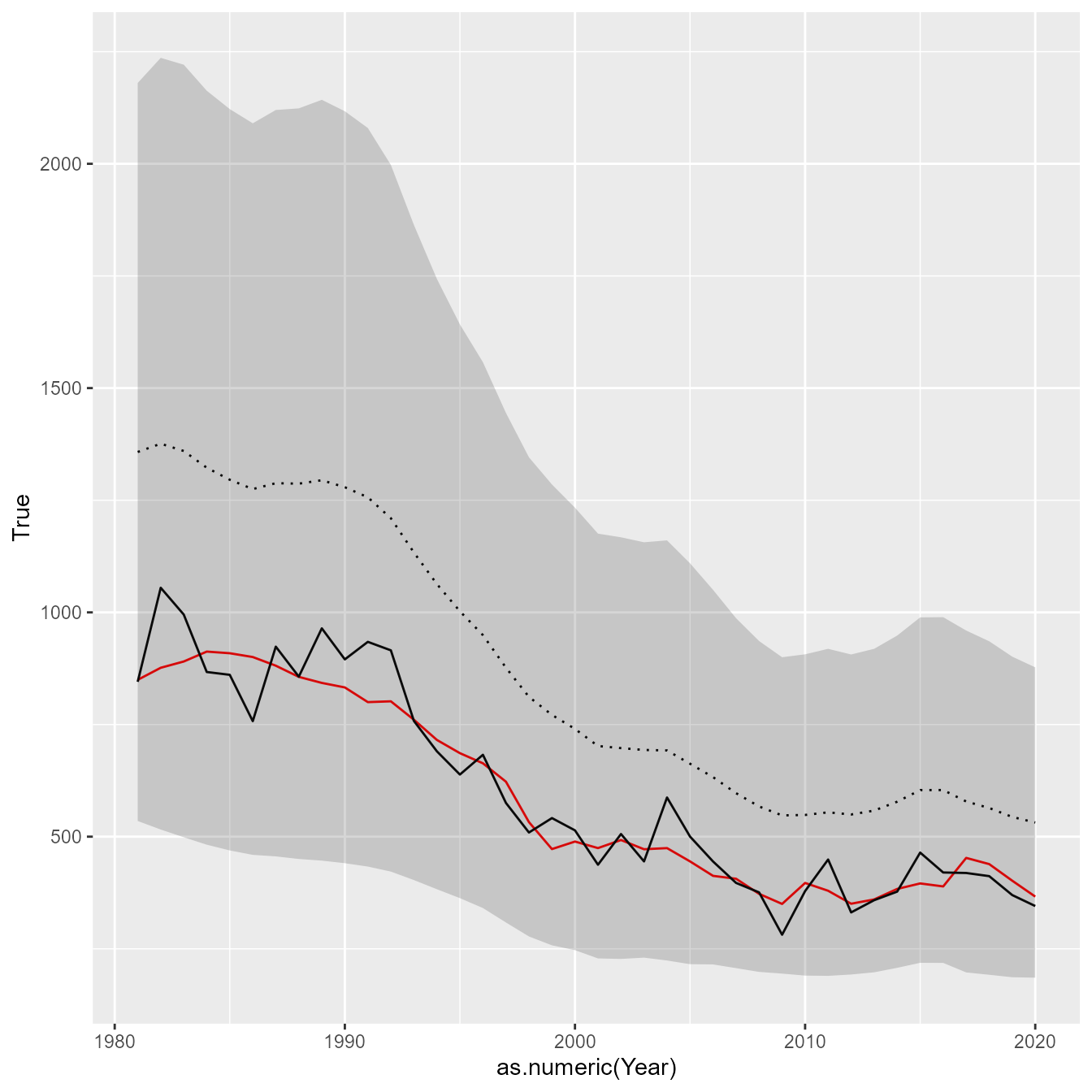

Bivariate production model

Similarly, we could fit a two-species production model to these same data:

# Inputs
taxa = c( "prey", "target" )
n_taxa = length(taxa)
PB_i = c( 5, 0.1 )
QB_i = c( NA, 0.5 )
DC_ij = matrix( c(0,0,1,0), nrow=2 )
X_ij = matrix( 2, nrow=2, ncol=2 )
U_i = c( 0.2, 0.2 )
type = c( "auto", "hetero" )
EE_i = c( 1, NA ) 
B_i = c( NA, 1 )

# Settings: specify what parameters to estimate
fit_eps = "target"   # process errors
fit_Q = "target"       # catchability coefficient
fit_B0 = c()      # non-equilibrium initial condition
fit_B = "target"       # equilibrium biomass

# Label EwE inputs for each taxon as expected (so users can easily change taxa)
names(PB_i) = names(QB_i) = names(B_i) = names(EE_i) = names(type) = names(U_i) = taxa
  dimnames(DC_ij) = dimnames(X_ij) = list("Prey"=taxa, "Predator"=taxa)
  
# Define priors
log_prior = function(p){
  # Prior on process-error log-SD to stabilize model
  logp = dnorm( p$logtau_i, mean=log(0.2), sd=1, log=TRUE )
}

# Run model
out_bivar = ecostate( taxa = taxa,
                years = years,
                catch = Catch,
                biomass = Biomass,
                PB = PB_i,
                QB = QB_i,
                DC = DC_ij,
                B = B_i,
                EE = EE_i,
                X = X_ij,
                type = type,
                U = U_i,
                fit_B = fit_B,
                fit_Q = fit_Q,
                fit_eps = fit_eps,
                fit_B0 = fit_B0,
                log_prior = log_prior,
                control = ecostate_control() )

# print output to terminal
out_bivar
#> Dynamics integrated using  ABM  with  10  time-steps
#> Run time: Time difference of 44.77589 secs
#> Negative log-likelihood: -75.16433
#> 
#> EcoSim parameters:
#>          type  QB  PB         B EE   U
#> prey     auto  NA 5.0  81.99584  1 0.2
#> target hetero 0.5 0.1 819.95841  0 0.2
#> 
#> EcoSim diet matrix:
#>         Predator
#> Prey     prey target
#>   prey      0      1
#>   target    0      0
#> 
#> EcoSim vulnerability matrix:
#>         Predator
#> Prey     prey target
#>   prey      2      2
#>   target    2      2
#> 
#> Estimates: sdreport(.) result
#>            Estimate Std. Error
#> logB_i    6.7092536  0.0935837
#> logtau_i -2.6240934  0.2387366
#> logq_i    0.1161167  0.1428179
#> Maximum gradient component: 1.10751e-05

We can then calculate and visualize how this changes the production function:

# Calculate annualized production function
yhat_bivar = sapply( x, FUN=prod_fun, ecofit=out_bivar, taxon="target",
               Xprime = out_bivar$internal$parhat$Xprime_ij, 
               logPB = out_bivar$internal$parhat$logPB_i )

# Empirical
phi_bivar = x[which.max(yhat_bivar)] / 1000 
msy_bivar = yhat_bivar[which.max(yhat_bivar)]


# Plot them
plot( x=x, y=y, type="l", xlim=c(0,2*K), ylim=c(0,2*max(y)), lwd=3, 
      xlab="Biomass", ylab="Annual surplus production" )
matplot( x=x, y=cbind(yhat,yhat_bivar), lwd=3, col=c("red","blue"), 
         type="l", add=TRUE )  
legend( "topright", fill=c("black","red","blue"), 
        legend=c("True","1-species","2-species"), bty="n")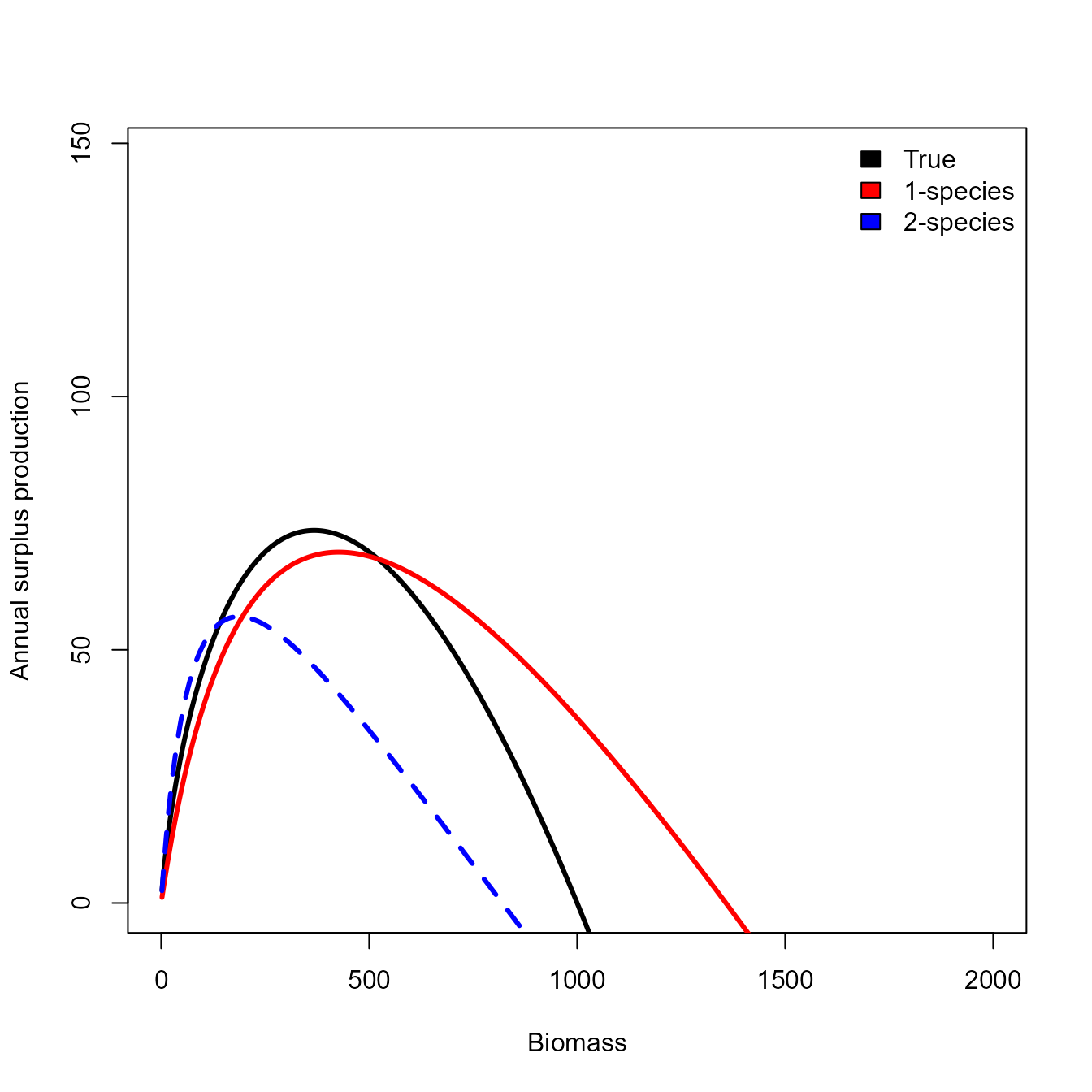

Age-structured model

Additionally, we could fit this model while also tracking abundance, average weight, and consumption for each age of the target species. We do this by including a single stanza. This then allows us to extract a time-series of average age and average weight.

# Inputs
taxa = c( "prey", "target" )
n_taxa = length(taxa)
PB_i = c( 5, 0.1 )
QB_i = c( NA, 0.5 )
DC_ij = matrix( c(0,0,1,0), nrow=2 )
X_ij = matrix( 2, nrow=2, ncol=2 )
U_i = c( 0.2, 0.2 )
type = c( "auto", "hetero" )
EE_i = c( 1, NA ) 
B_i = c( NA, 1 )

# Settings: specify what parameters to estimate
fit_eps = "target"   # process errors
fit_Q = "target"       # catchability coefficient
fit_B0 = c()      # non-equilibrium initial condition
fit_B = "target"       # equilibrium biomass

# Label EwE inputs for each taxon as expected (so users can easily change taxa)
names(PB_i) = names(QB_i) = names(B_i) = names(EE_i) = names(type) = names(U_i) = taxa
  dimnames(DC_ij) = dimnames(X_ij) = list("Prey"=taxa, "Predator"=taxa)
  
# Define priors
log_prior = function(p){
  # Prior on process-error log-SD to stabilize model
  logp = dnorm( p$logtau_i, mean=log(0.2), sd=1, log=TRUE )
}

# Run model
out_stanzas = ecostate( taxa = taxa,
                years = years,
                catch = Catch,
                biomass = Biomass,
                PB = PB_i,
                QB = QB_i,
                DC = DC_ij,
                B = B_i,
                EE = EE_i,
                X = X_ij,
                type = type,
                U = U_i,
                fit_B = fit_B,
                fit_Q = fit_Q,
                fit_eps = fit_eps,
                fit_B0 = fit_B0,
                control = ecostate_control(),
                log_prior = log_prior,
                settings = stanza_settings( taxa = taxa,
                                            stanza_groups = c("target"="age_structured"),
                                            K = c("age_structured" = 0.1),
                                            Wmat = c("age_structured" = (2/3)^3),
                                            d = c("age_structured" = 2/3),
                                            Amax = c("target" = 30),
                                            SpawnX = c("age_structured" = 2)
                                           ))

# print output to terminal
out_stanzas
#> Dynamics integrated using  ABM  with  10  time-steps
#> Run time: Time difference of 54.95873 secs
#> Negative log-likelihood: -71.35349
#> 
#> EcoSim parameters:
#>          type  QB  PB         B EE   U
#> prey     auto  NA 5.0  104.2852  1 0.2
#> target hetero 0.5 0.1 1042.8523  0 0.2
#> 
#> EcoSim diet matrix:
#>         Predator
#> Prey     prey target
#>   prey      0      1
#>   target    0      0
#> 
#> EcoSim vulnerability matrix:
#>         Predator
#> Prey     prey target
#>   prey      2      2
#>   target    2      2
#> 
#> Estimates: sdreport(.) result
#>            Estimate Std. Error
#> logB_i    6.9497148 0.02793407
#> logtau_i -3.1538949 0.50332833
#> logq_i   -0.1443941 0.04695328
#> Maximum gradient component: 0.0002864114

#
meanage_t = meanweight_t = rep(NA, length(years))
for(t in seq_along(years)){
  meanage_t[t] = weighted.mean( x = 1:30,
                                w = exp(out_stanzas$rep$Y_tzz_g2[[1]][t,,'log_NageS']) )
  meanweight_t[t] = weighted.mean( x = out_stanzas$rep$Y_tzz_g2[[1]][t,,'WageS'],
                                   w = exp(out_stanzas$rep$Y_tzz_g2[[1]][t,,'log_NageS']) )
}
par( mfrow=c(2,1), mar=c(3,4,2,1) )
plot( x=years, y=meanage_t, lwd=2, type="l", main="Mean age" )
plot( x=years, y=meanweight_t, lwd=2, type="l", main="Mean weight" )

In this age-structured production model, mean age decreases with increased fishing, but mean weight increases due to compensatory growth as the ratio of forage to predator increases.

Multi-stanza age-structured production model

Finally, we could fit a model with three variables, representing a forage species and two age-structured “stanzas” for the focal species. Here, we specify identical diet but varying bioenergetics by size:

# Inputs
taxa = c( "prey", "stage1", "stage2" )
n_taxa = length(taxa)
PB_i = c( 5, 1, 0.1 )
QB_i = c( NA, NA, 0.5 )
DC_ij = cbind( "prey"=c(0,0,0), "stage1"=c(1,0,0), "stage2"=c(1,0,0)  )
X_ij = matrix( 2, nrow=length(taxa), ncol=length(taxa) )
U_i = c( 0.2, 0.2, 0.2 )
type = c( "auto", "hetero", "hetero" )
EE_i = c( 1, NA, NA ) 
B_i = c( NA, NA, 1 )

# Settings: specify what parameters to estimate
fit_eps = c("stage1","stage2")   # process errors
fit_Q = "stage2"       # catchability coefficient
fit_B0 = c()      # non-equilibrium initial condition
fit_B = "stage2"       # equilibrium biomass

# Label EwE inputs for each taxon as expected (so users can easily change taxa)
names(PB_i) = names(QB_i) = names(B_i) = names(EE_i) = names(type) = names(U_i) = taxa
  dimnames(DC_ij) = dimnames(X_ij) = list("Prey"=taxa, "Predator"=taxa)

# Define priors
log_prior = function(p){
  # Prior on process-error log-SD to stabilize model
  logp = sum(dnorm( p$logtau_i[2:3], mean=log(0.2), sd=1, log=TRUE))
}

# Run model
out_trivar = ecostate( 
  taxa = taxa,
  years = years,
  catch = data.frame("Mass"=Catch[,1],"Year"=Catch[,2],"Taxon"="stage2"),
  biomass = data.frame("Mass"=Biomass[,1],"Year"=Biomass[,2],"Taxon"="stage2"),
  PB = PB_i,
  QB = QB_i,
  DC = DC_ij,
  B = B_i,
  EE = EE_i,
  X = X_ij,
  type = type,
  U = U_i,
  fit_B = fit_B,
  fit_Q = fit_Q,
  fit_eps = fit_eps,
  fit_B0 = fit_B0,
  log_prior = log_prior,
  control = ecostate_control(),
  settings = stanza_settings( 
    taxa = taxa,
    stanza_groups = c("stage1"="age_structured", "stage2"="age_structured"),
    K = c("age_structured" = 0.1),
    Wmat = c("age_structured" = (2/3)^3),
    d = c("age_structured" = 2/3),
    Amax = c("stage1" = 2, "stage2" = 30),
    SpawnX = c("age_structured" = 2) )
)
#> Warning in nlminb(start = opt$par, objective = obj$fn, gradient = list(obj$gr,
#> : NA/NaN function evaluation

# print output to terminal
out_trivar
#> Dynamics integrated using  ABM  with  10  time-steps
#> Run time: Time difference of 2.824025 mins
#> Negative log-likelihood: -70.41958
#> 
#> EcoSim parameters:
#>          type       QB  PB            B EE   U
#> prey     auto       NA 5.0  106.7457516  1 0.2
#> stage1 hetero 3.916939 1.0    0.8281451  0 0.2
#> stage2 hetero 0.500000 0.1 1060.9699286  0 0.2
#> 
#> EcoSim diet matrix:
#>         Predator
#> Prey     prey stage1 stage2
#>   prey      0      1      1
#>   stage1    0      0      0
#>   stage2    0      0      0
#> 
#> EcoSim vulnerability matrix:
#>         Predator
#> Prey     prey stage1 stage2
#>   prey      2      2      2
#>   stage1    2      2      2
#>   stage2    2      2      2
#> 
#> Estimates: sdreport(.) result
#>            Estimate Std. Error
#> logB_i    6.9669388 0.08521457
#> logtau_i  0.3498846 0.37557231
#> logtau_i -3.1440545 0.50456842
#> logq_i   -0.1292594 0.09806604
#> Maximum gradient component: 1.809354e-09

The model includes process-errors in the first-stage (eggs to recruits, from age-0 to age-2) and the second stage (age-2 onward), although the variance for stage-1 collapses to zero in this simulation replicate.

Comparison with other models

We can compare this with a state-space production model in continuous time (SPiCT):

# Format for SPiCT
datalist = list(
  obsC = C_t[-1],
  timeC = years[-1],
  obsI = Bobs_t,
  timeI = years              
)

# Fit and plot
res <- fit.spict(datalist)
plotspict.biomass(res)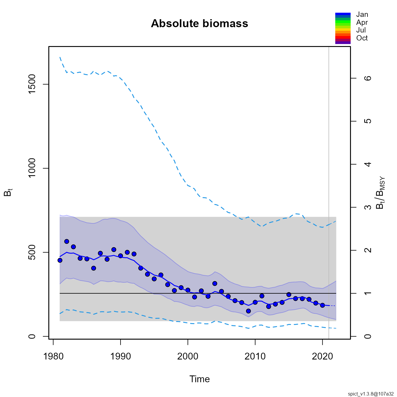

Similarly, we can compare it with Just Another Bayesian Biomass Assessment (JABBA):

# Compile JABBA JAGS model and input object
jbinput = build_jabba( catch = data.frame(Year=years, Total=C_t)[-1,],
                       cpue = data.frame(Year=years, Index=Bobs_t)[-1,],
                       se = data.frame(Year=years, Index=0.1)[-1,],
                       assessment = "target",
                       scenario = "TestRun",
                       model.type = "Schaefer",
                       sigma.est = FALSE,
                       fixed.obsE = 0.1 )
#> 
#> ><> Prepare JABBA input data <><
#> 
#> ><> Assume Catch with error CV = 0.1 <><
#> 
#> ><> Model type:Schaefer <><
#> 
#> ><> Shape m =2
#> 
#> ><> K prior mean =888.164844109276and CV =1(log.sd = 0.832554611157698)
#> 
#> ><> r prior mean =0.2and CV =0.532940350027788(log.sd = 0.5)
#> 
#> ><> Psi (B1/K) prior mean =0.9and CV =0.25withlnormdestribution
#> 
#> 
#> 
#> ><> ALWAYS ENSURE to adjust default settings to your specific stock <><

# Fit JABBA (here mostly default value - careful)
bet1 = fit_jabba(jbinput, quickmcmc=TRUE)
#> module glm loaded
#> Compiling model graph
#>    Resolving undeclared variables
#>    Allocating nodes
#> Graph information:
#>    Observed stochastic nodes: 120
#>    Unobserved stochastic nodes: 124
#>    Total graph size: 2169
#> 
#> Initializing model
#> 
#> ><> Produce results output of Schaefer model for target TestRun <><
#> 
#> 
#> ><> Scenario TestRun_Schaefer completed in 0 min and 35 sec <><

# Make individual plots
jbplot_cpuefits(bet1)
#> 
#> ><> jbplot_cpue() - fits to CPUE <><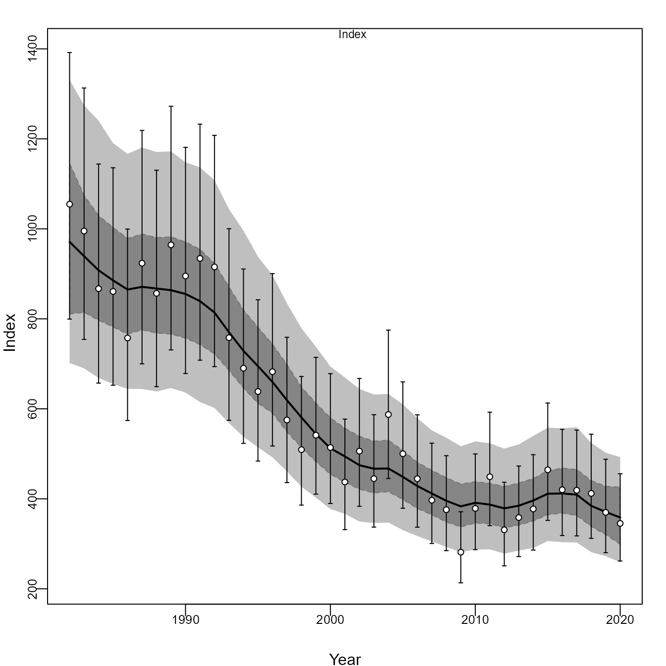

Comparing the two shows that SPICT, JABBA, and all configurations of EcoState have errors in estimating population scale, presumably due to mis-specifying the production function. As expected, the age-structured and 2-species EcoState models result in identical estimates, where the age-structured version also provides auxiliary information about changes in average age and size.

# Compare estimates
knitr::kable(rbind(
  "True" = c("q" = q, "K"=K, "MSY"=true_msy),
  "EcoState 1-species" = c(exp(out$opt$par[c('logq_i','logB_i')]),msy2),
  "EcoState 2-species" = c(exp(out_bivar$opt$par[c('logq_i','logB_i')]),msy_bivar),
  "EcoState age-structured" = c(exp(out_stanzas$opt$par[c('logq_i','logB_i')]),NA),
  "EcoState multi-stanza" = c(exp(out_trivar$opt$par[c('logq_i','logB_i')]),NA),
  "SPiCT" = c(res$value[c('q','K','MSY')]),
  "JABBA" = c(bet1$pars[c('q','K'),'Median'],bet1$estimates['MSY','mu'])
), digits=3)

	q	K	MSY
True	1.000	1000.000	73.576
EcoState 1-species	0.685	1357.543	69.279
EcoState 2-species	1.123	819.958	56.546
EcoState age-structured	0.866	1042.852	NA
EcoState multi-stanza	0.879	1060.970	NA
SPiCT	1.868	508.147	76.990
JABBA	0.728	1222.962	68.805

Runtime for this vignette: 5.41 mins

James Thorson

Simulation demonstration

Bivariate production model

Age-structured model

Multi-stanza age-structured production model

Comparison with other models