Demonstrating EcoState via simulation
James Thorson
Source:vignettes/not_on_cran/simulation.Rmd
simulation.Rmdecostate is an R package for fitting the mass-balance
dynamics specified by EcoSim as a state-space model. We here highlight a
few features in particular.
Simulation demonstration
W begin by specifying parameters for a 5-species ecosystem:
# Time-interval
years = 1981:2020
n_years = length(years)

# Name taxa (optional, for illustration)
taxa = c("Consumer_1", "Consumer_2", "Predator_1", "Predator_2", "Producer", "Detritus")
n_species = length(taxa)

# Type for each taxon
type_i = c( "hetero", "hetero", "hetero", "hetero", "auto", "detritus" )

# Diet matrix
DC_ij = matrix( c(
  0,     0,     0.8,  0.4,  0,   0,
  0,     0,     0.2,  0.6,  0,   0,
  0,     0,     0,    0,    0,   0,
  0,     0,     0,    0,    0,   0,
  0.9,   0.3,   0,    0,    0,   0,
  0.1,   0.7,   0,    0,    0,   0
), byrow=TRUE, ncol=n_species)

# Reciprocal of mean age according to Polovina-1984 ~= M
PB_i = c( 4, 1, 0.2, 0.1, 90, 0.5 )

# Consumption per biomass for heterotrophcs
QB_i = c( 10, 4, 3, 1, NA, NA )

# Define ecotrophic efficiency or biomass for each taxon
EE_i = c( 0.9, 0.9, NA, NA, 0.9, 0.9 )
B_i = c( NA, NA, 1, 1, NA, NA )

# Unassimulated food
U_i = rep( 0.2, n_species )

# Vulnerability matrix
X_ij = matrix( 2, nrow=n_species, ncol=n_species )
X_ij[,which(type_i=="auto")] = 91

# Label EwE inputs for each taxon as expected (so users can easily change taxa)
names(PB_i) = names(QB_i) = names(type_i) = names(U_i) = names(B_i) = names(EE_i) = taxa
  dimnames(DC_ij) = dimnames(X_ij) = list("Prey"=taxa, "Predator"=taxa)
We can then simulate data using the same functions for mass-balance and simulating dynamics are then used by EcoState during parameter estimation:
# Define Biomass for Taxon-Year combinations with survey data
Biomass = cbind( expand.grid( "Year" = years,
                           "Taxon" = taxa ),
               "Mass" = 1 )

# Define catch for Taxon-Year combinations with a fishery
Catch = subset( Biomass, Taxon %in% c("Predator_1","Predator_2") )

# Build the model object
out = ecostate( taxa = taxa,
                years = years,
                catch = Catch,
                biomass = Biomass,
                PB = PB_i,
                QB = QB_i,
                DC = DC_ij,
                B = B_i,
                EE = EE_i,
                X = X_ij,
                type = type_i,
                U = U_i,
                control = ecostate_control( nlminb_loops = 0,
                                            getsd = 0 ))

# Edit the parameters used
parlist = out$obj$env$parList()
# Fishing mortality for Predator_1
parlist$logF_ti[,3] = log( 0.2 * seq(0, 1, len=n_years) )
# Fishing mortality for Predator_2
parlist$logF_ti[,4] = log( 0.1 * seq(0, 1, len=n_years) )

# print output to terminal
sim = out$simulator( parlist = parlist )
Comparison with Rpath
We first compare the functions used by EcoState with existing implementations of the model. One script-based implementation available in R is Rpath, and we therefore show the syntax and model-output for this comparison.
For this comparison, we first load Rpath and reformat
inputs in the format that it expects to calculate mass-balance:
# Rpath needs types in ascending order (EcoState doesn't care)
types  <- sapply( c(type_i,"fishery"), FUN=switch,
                  "hetero"==0, "auto"=1, "detritus"=2, "fishery"=3 )
groups <- c( taxa, "fishery" )
stgroups = rep(NA, length(groups) )
REco.params <- create.rpath.params(group = groups, type = types, stgroup = stgroups)

# Fill in biomass
#REco.params$model$Biomass = c( exp(Pars_full$logB_i), NA )
REco.params$model$Biomass = c( B_i, NA )
REco.params$model$EE = c( ifelse(type_i=="detritus",NA,EE_i), NA )
REco.params$model$PB = c( PB_i, NA )
REco.params$model$QB = c( QB_i, NA )

#Biomass accumulation and unassimilated consumption
REco.params$model$BioAcc = c( rep(0,length(taxa)), NA )
REco.params$model$Unassim = c( ifelse(type_i=="hetero",0.2,0), NA )

#Detrital Fate
REco.params$model$Detritus = c( ifelse(type_i=="detritus",0,1), 0 )
REco.params$model$fishery = c( rep(0,length(taxa)), NA )
REco.params$model$fishery.disc = c( rep(0,length(taxa)), NA )

# Diet
for(j in 1:5) REco.params$diet[seq_along(taxa),j+1] = DC_ij[,j]
REco.params$diet[seq_along(taxa),2] = DC_ij[,1]

# Balance using Ecopath equations
check.rpath.params( REco.params)
#> Rpath parameter file is functional.
REco <- rpath(REco.params, eco.name = 'R Ecosystem')
We can then simulate forward in time using Rpath:
# Create simulation object
REco.sim <- rsim.scenario(REco, REco.params, years = 1:40)

#
REco.sim = adjust.fishing( Rsim.scenario=REco.sim,
                           parameter='ForcedFRate',
                           group = 'Predator_1', # Group is which species to apply
                           sim.year = 1:40,
                           sim.month = 0,
                           value = (1:40/40)*0.2 )
REco.sim = adjust.fishing( Rsim.scenario=REco.sim,
                           parameter='ForcedFRate',
                           group = 'Predator_2', # Group is which species to apply
                           sim.year = 1:40,
                           sim.month = 0,
                           value = (1:40/40)*0.1 )

# Match vulnerability for self-limitation in Producers
REco.sim$params$VV[which(REco.sim$params$PreyFrom==0 & REco.sim$params$PreyTo==5)] = 91

#
REco.run1 <- rsim.run(REco.sim, method = 'RK4', years = 1:40)
Simulate using Ecostate
Comparing the scenario forecasted with Rpath against the simulated time-series, we see that the two closely match. EcoState uses the same functions during fitting, and so it also closely matches Rpath.
# Calculate annual simulated catch
Year = rep( years, each=12)
Bsim_ti = apply( REco.run1$out_Biomass[,-1], MARGIN=2, FUN=\(x) tapply(x,INDEX=Year,FUN=mean) )

#
par(mfrow=c(2,1), mar=c(3,3,1,1), mgp=c(2,0.5,0) )
matplot( x=years, y=Bsim_ti / outer(rep(1,n_years),Bsim_ti[1,]),
         type="l", lwd=3, lty="solid", col=rainbow(n_species), log="y",
         ylab="Relative biomass (Rpath)", xlab="Year" )
Brel_ti = sim$B_ti / outer(rep(1,n_years),sim$B_ti[1,])
matplot( x=years, y=sim$B_ti / outer(rep(1,n_years),sim$B_ti[1,]),
         type="l", lwd=3, lty="solid", col=rainbow(n_species), log="y",
         ylab="Relative biomass (Simulated)", xlab="Year" )
legend("bottomleft", fill=rainbow(n_species), legend=taxa, ncol=2, bty="n")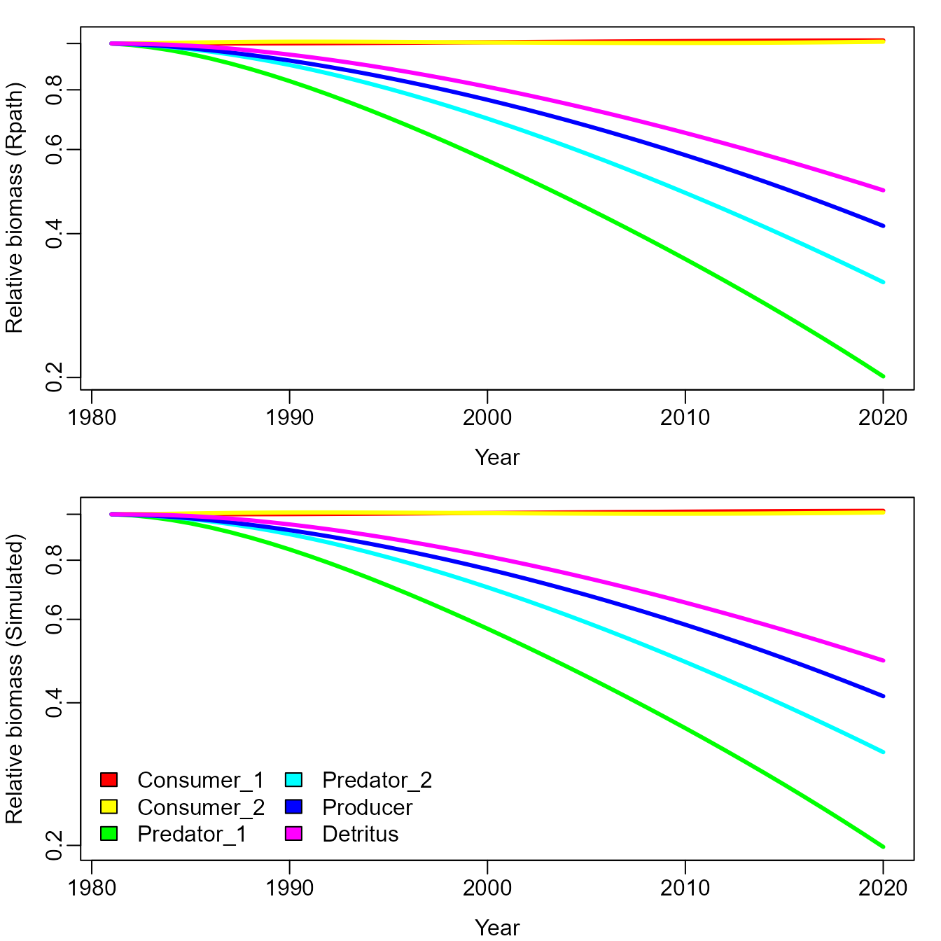
Fitting the model using EcoState
We next want to show how EcoState performs when fitting to simulated data. We first rebuild the model with process errors, and simulate new data
and plot it to compare with the previous simulation that did not have process errors:
# Build the model object
out = ecostate( taxa = taxa,
                years = years,
                catch = Catch,
                biomass = Biomass,
                PB = PB_i,
                QB = QB_i,
                DC = DC_ij,
                B = B_i,
                EE = EE_i,
                X = X_ij,
                type = type_i,
                U = U_i,
                fit_eps = taxa,
                control = ecostate_control( nlminb_loops = 0,
                                            getsd = 0 ))

# Simulate new data
#sigmaB_i = c(0.02, 0.02, 0.1, 0.1, 0.1, 0.1) # Taxa 1-2 crashes solver if sigmaB > 0.02
#sim = simulate_data()

# Edit the parameters used
parlist = out$obj$env$parList()
# Fishing mortality for Predator_1
parlist$logF_ti[,3] = log( 0.2 * seq(0, 1, len=n_years) )
# Fishing mortality for Predator_2
parlist$logF_ti[,4] = log( 0.1 * seq(0, 1, len=n_years) )
# standard deviation for process errors in biomass dynamics
parlist$logtau_i = log(c(0.02, 0.02, 0.1, 0.1, 0.1, 0.1))

# print output to terminal
sim = out$simulator( parlist = parlist )

# Unload simulated data
Bobs_ti = sim$Bobs_ti
Cobs_ti = sim$Cobs_ti
B_ti = sim$B_ti

# Plot simulation with process errors
matplot( x=years, y=B_ti / outer(rep(1,n_years),B_ti[1,]),
         type="l", lwd=3, lty="solid", col=rainbow(n_species), log="y",
         ylab="Relative biomass (simulated)", xlab="Year" )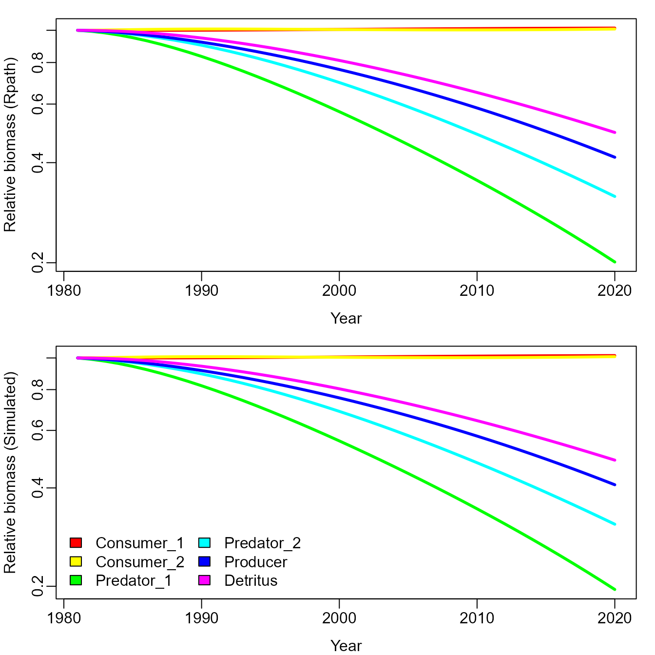
We then reformat simulated biomass and catch time-series into
long-form data frames and fit them with ecostate
# reformat to longform data-frame
Catch = na.omit( data.frame( expand.grid( "Year" = rownames(sim$Cobs_ti),
                                          "Taxon" = colnames(sim$Cobs_ti)),
                 "Mass"=as.vector(sim$Cobs_ti)))
Biomass = data.frame( expand.grid( "Year" = rownames(sim$Bobs_ti),
                                          "Taxon" = colnames(sim$Bobs_ti)),
                 "Mass"=as.vector(sim$Bobs_ti))

# Settings: specify what parameters to estimate
fit_eps = c("Producer", "Detritus", "Predator_1", "Predator_2")   # process errors
fit_Q = c()       # catchability coefficient
fit_B0 = c()      # non-equilibrium initial condition
fit_B = taxa       # equilibrium biomass

# Solving for EE and giving uninformed initial values for biomass
fittedB_i = sim$Bobs_ti[1,]
fittedEE_i = rep(NA, n_species)
names(fittedB_i) = names(fittedEE_i) = taxa

# Define priors
log_prior = function(p){
  # Prior on process-error log-SD to stabilize model
  logp = sum(dnorm( p$logtau_i, mean=log(0.2), sd=1, log=TRUE ), na.rm=TRUE)
}

# Run model
out = ecostate( taxa = taxa,
                years = years,
                catch = Catch,
                biomass = Biomass,
                PB = PB_i,
                QB = QB_i,
                DC = DC_ij,
                B = fittedB_i,
                EE = fittedEE_i,
                X = X_ij,
                type = type_i,
                U = U_i,
                fit_B = fit_B,
                fit_Q = fit_Q,
                fit_eps = fit_eps,
                fit_B0 = fit_B0,
                log_prior = log_prior,
                control = ecostate_control( # Much faster to turn off
                                            tmbad.sparse_hessian_compress = 0,
                                            # Faster to profile these
                                            profile = c("logF_ti","logB_i"),
                                            # More stable when starting low
                                            start_tau = 0.001 ))

# print output to terminal
out
#> Dynamics integrated using  ABM  with  10  time-steps
#> Run time: Time difference of 2.04871 mins
#> Negative log-likelihood: -276.8183
#>
#> EcoSim parameters:
#>                type QB   PB          B        EE   U
#> Consumer_1   hetero 10  4.0  0.7861948 0.8787131 0.2
#> Consumer_2   hetero  4  1.0  1.3367890 0.8910455 0.2
#> Predator_1   hetero  3  0.2  0.9846327 0.0000000 0.2
#> Predator_2   hetero  1  0.1  1.0006005 0.0000000 0.2
#> Producer       auto NA 90.0  0.1037043 0.9299841 0.2
#> Detritus   detritus NA  0.5 10.0965041 0.8971826 0.2
#>
#> EcoSim diet matrix:
#>             Predator
#> Prey         Consumer_1 Consumer_2 Predator_1 Predator_2 Producer Detritus
#>   Consumer_1        0.0        0.0        0.8        0.4        0        0
#>   Consumer_2        0.0        0.0        0.2        0.6        0        0
#>   Predator_1        0.0        0.0        0.0        0.0        0        0
#>   Predator_2        0.0        0.0        0.0        0.0        0        0
#>   Producer          0.9        0.3        0.0        0.0        0        0
#>   Detritus          0.1        0.7        0.0        0.0        0        0
#>
#> EcoSim vulnerability matrix:
#>             Predator
#> Prey         Consumer_1 Consumer_2 Predator_1 Predator_2 Producer Detritus
#>   Consumer_1          2          2          2          2       91        2
#>   Consumer_2          2          2          2          2       91        2
#>   Predator_1          2          2          2          2       91        2
#>   Predator_2          2          2          2          2       91        2
#>   Producer            2          2          2          2       91        2
#>   Detritus            2          2          2          2       91        2
#>
#> Estimates: sdreport(.) result
#>           Estimate Std. Error
#> logtau_i -2.438964  0.2090417
#> logtau_i -3.158383  0.3105397
#> logtau_i -1.547155  0.9708793
#> logtau_i -2.254995  0.2185956
#> Maximum gradient component: 1.650295e-05
Finally, we can extract elements from the fitted model, and plot them easily using ggplot2 to compare them with known (simulated) values. This exercise shows that EcoState can accurately estimate biomass trends:
# Extract estimated biomass
Bhat_ti = out$derived$Est$B_ti
Bse_ti = out$derived$SE$B_ti

# Reformat to long-form data frame for ggplot
results = expand.grid( "Year" = years, "Taxon" = taxa )
results = cbind( results,
                 "True" = as.vector(B_ti),
                 "Est" = as.vector(Bhat_ti),
                 "SE" = as.vector(Bse_ti) )

# Plot using ggplot
library(ggplot2)
ggplot(results) +
  geom_line( aes(x=as.numeric(Year), y=True) ) +
  facet_wrap( vars(Taxon), scale="free" ) +
  geom_line( aes(x=as.numeric(Year), y=Est), linetype="dotted" ) +
geom_ribbon( aes(x=as.numeric(Year), ymin=Est-SE, ymax=Est+SE), alpha=0.2) 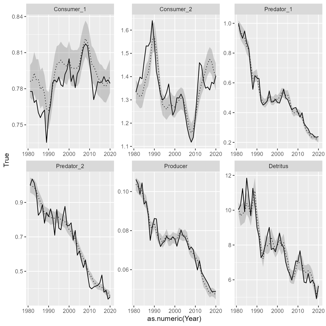
Advanced: estimating vulnerability parameters
We can also explore estimating additional parameters. Here, we explore estimating vulnerability:
# Define priors
log_prior = function(p){
  # Prior on process-error log-SD to stabilize model
  logp = sum(dnorm( p$logtau_i, mean=log(0.2), sd=1, log=TRUE ), na.rm=TRUE)
  # Prior on vulnerability to stabilize model (single value mirrored below)
  logp = logp + dnorm( p$Xprime_ij[1,1], mean=0, sd=1, log=TRUE )
}

# Run model
out0 = ecostate( taxa = taxa,
                years = years,
                catch = Catch,
                biomass = Biomass,
                PB = PB_i,
                QB = QB_i,
                DC = DC_ij,
                B = fittedB_i,
                EE = fittedEE_i,
                X = X_ij,
                type = type_i,
                U = U_i,
                fit_B = fit_B,
                fit_Q = fit_Q,
                fit_eps = fit_eps,
                fit_B0 = fit_B0,
                log_prior = log_prior,
                control = ecostate_control( inverse_method = "Standard",
                                            nlminb_loops = 0,
                                            tmbad.sparse_hessian_compress = 0,
                                            getsd = FALSE,
                                            process_error = "epsilon",
                                            profile = c("logF_ti","logB_i"),
                                            start_tau = 0.1 ))

# Change tmb_par
tmb_par = out0$tmb_inputs$p
  tmb_par$Xprime_ij[,which(type_i!="auto")] = log(1.5 - 1)
map = out0$tmb_inputs$map
  map$Xprime_ij = array(NA, dim=dim(tmb_par$Xprime_ij))
  map$Xprime_ij[,which(type_i!="auto")] = 1
  map$Xprime_ij = factor(map$Xprime_ij)

# Run model
out = ecostate( taxa = taxa,
                years = years,
                catch = Catch,
                biomass = Biomass,
                PB = PB_i,
                QB = QB_i,
                DC = DC_ij,
                B = fittedB_i,
                EE = fittedEE_i,
                X = X_ij,
                type = type_i,
                U = U_i,
                fit_B = fit_B,
                fit_Q = fit_Q,
                fit_eps = fit_eps,
                fit_B0 = fit_B0,
                log_prior = log_prior,
                control = ecostate_control( inverse_method = "Standard",
                                            nlminb_loops = 1,
                                            tmbad.sparse_hessian_compress = 0,
                                            getsd = TRUE,
                                            process_error = "epsilon",
                                            profile = c("logF_ti","logB_i"),
                                            start_tau = 0.001,
                                            tmb_par = tmb_par,
                                            map = map ))   # alpha is faster than epsilon
#> Using `control$tmb_par`, so be cautious in constructing it
#> Using `control$map`, so be cautious in constructing it

# print output to terminal
out
#> Dynamics integrated using  ABM  with  10  time-steps
#> Run time: Time difference of 2.103908 mins
#> Negative log-likelihood: -275.9045
#>
#> EcoSim parameters:
#>                type QB   PB          B        EE   U
#> Consumer_1   hetero 10  4.0  0.7861405 0.8797942 0.2
#> Consumer_2   hetero  4  1.0  1.3365146 0.8920989 0.2
#> Predator_1   hetero  3  0.2  0.9858493 0.0000000 0.2
#> Predator_2   hetero  1  0.1  1.0013227 0.0000000 0.2
#> Producer       auto NA 90.0  0.1035994 0.9308375 0.2
#> Detritus   detritus NA  0.5 10.0885570 0.8977263 0.2
#>
#> EcoSim diet matrix:
#>             Predator
#> Prey         Consumer_1 Consumer_2 Predator_1 Predator_2 Producer Detritus
#>   Consumer_1        0.0        0.0        0.8        0.4        0        0
#>   Consumer_2        0.0        0.0        0.2        0.6        0        0
#>   Predator_1        0.0        0.0        0.0        0.0        0        0
#>   Predator_2        0.0        0.0        0.0        0.0        0        0
#>   Producer          0.9        0.3        0.0        0.0        0        0
#>   Detritus          0.1        0.7        0.0        0.0        0        0
#>
#> EcoSim vulnerability matrix:
#>             Predator
#> Prey         Consumer_1 Consumer_2 Predator_1 Predator_2 Producer Detritus
#>   Consumer_1   1.983361   1.983361   1.983361   1.983361       91 1.983361
#>   Consumer_2   1.983361   1.983361   1.983361   1.983361       91 1.983361
#>   Predator_1   1.983361   1.983361   1.983361   1.983361       91 1.983361
#>   Predator_2   1.983361   1.983361   1.983361   1.983361       91 1.983361
#>   Producer     1.983361   1.983361   1.983361   1.983361       91 1.983361
#>   Detritus     1.983361   1.983361   1.983361   1.983361       91 1.983361
#>
#> Estimates: sdreport(.) result
#>              Estimate Std. Error
#> Xprime_ij -0.01677909  0.1636022
#> logtau_i  -2.43903330  0.2091244
#> logtau_i  -3.16204128  0.3134125
#> logtau_i  -1.54955378  0.9719704
#> logtau_i  -2.25520900  0.2186404
#> Maximum gradient component: 9.629189e-07
Runtime for this vignette: 4.27 mins