Model of Intermediate Complexity

library(ecostate)

ecostate is an R package for fitting the mass-balance dynamics specified by EcoSim as a state-space model. We here demonstrate how it can be fitted to a real-world data set as a “Model of Intermediate Complexity” while including 10 functional groups and 1 detritus pool, using data across four trophic levels and representing both pelagic and demersal energy pathways.

Eastern Bering Sea

We first load the Survey, Catch, PB, and QB values, and define other biological inputs:

# load data
data(eastern_bering_sea)

# Reformat inputs
years = 1982:2021 # Catch only goes through 2021, and starting pre-data in 1982 doesn't play well with fit_B0
taxa = c( "Pollock", "Cod", "Arrowtooth", "Copepod", "Other_zoop", "Chloro", "NFS", "Krill", "Benthic_invert", "Benthos", "Detritus" )

# Define types
type_i = sapply( taxa, FUN=switch, "Detritus" = "detritus",
                                   "Chloro" = "auto",
                                   "hetero" )

# Starting values
U_i = EE_i = B_i = array( NA, dim=length(taxa), 
                    dimnames=list(names(eastern_bering_sea$P_over_B)))
B_i[c("Cod", "Arrowtooth", "NFS")] = c(1, 0.5, 0.02)
EE_i[] = 1
U_i[] = 0.2

# Define default vulnerability, except for primary producers
X_ij = array( 2, dim=c(length(taxa),length(taxa)) )
dimnames(X_ij) = list(names(B_i),names(B_i))
X_ij[,'Chloro'] = 91

We then fit the function call. This is very slow:

# Define parameters to estimate
fit_Q = c("Pollock", "Copepod", "Chloro", "Other_zoop", "Krill")
fit_B0 = c("Pollock", "Cod", "Arrowtooth", "NFS")
fit_B = c("Cod", "Arrowtooth", "NFS")  

# Define process errors to estimate
# Only estimating Pollock to speed up demonstration
fit_eps = "Pollock"

# Which taxa to include
taxa_to_include = c( "NFS", "Pollock", "Copepod", "Chloro", "Krill" )
# To run full model use:
# taxa_to_include = taxa

# Define priors
log_prior = function(p){
  # Prior on process-error log-SD to stabilize model
  logp = sum(dnorm( p$logtau_i, mean=log(0.2), sd=1, log=TRUE ), na.rm=TRUE)
}

# Run model
out = ecostate( taxa = taxa_to_include,
                years = years,
                catch = eastern_bering_sea$Catch,
                biomass = eastern_bering_sea$Survey,
                PB = eastern_bering_sea$P_over_B,
                QB = eastern_bering_sea$Q_over_B,
                DC = eastern_bering_sea$Diet_proportions,
                B = B_i,
                EE = EE_i,
                U = U_i,
                type = type_i,
                X = X_ij,
                fit_B = fit_B,
                fit_Q = fit_Q,
                fit_eps = fit_eps,
                fit_B0 = fit_B0,
                log_prior = log_prior,
                control = ecostate_control( n_steps = 20, # using 15 by default
                                            start_tau = 0.01,
                                            tmbad.sparse_hessian_compress = 0 ))

# print output
out
#> Dynamics integrated using  ABM  with  20  time-steps
#> Run time: Time difference of 3.061711 mins
#> Negative log-likelihood: 111.8524
#> 
#> EcoSim parameters:
#>           type        QB          PB          B EE   U
#> NFS     hetero 57.763550  0.09429851 0.01609925  0 0.2
#> Pollock hetero  4.225892  0.82452074 3.26652224  1 0.2
#> Copepod hetero 27.740000  6.00000000 1.85225167  1 0.2
#> Chloro    auto        NA 99.40685006 0.63388263  1 0.2
#> Krill   hetero 15.640000  5.48000000 1.05351582  1 0.2
#> 
#> EcoSim diet matrix:
#>          Predator
#> Prey      NFS   Pollock Copepod Chloro     Krill
#>   NFS       0 0.0000000       0      0 0.0000000
#>   Pollock   1 0.1277434       0      0 0.0000000
#>   Copepod   0 0.4540243       0      0 0.2941176
#>   Chloro    0 0.0000000       1      0 0.7058824
#>   Krill     0 0.4182324       0      0 0.0000000
#> 
#> EcoSim vulnerability matrix:
#>         NFS Pollock Copepod Chloro Krill
#> NFS       2       2       2     91     2
#> Pollock   2       2       2     91     2
#> Copepod   2       2       2     91     2
#> Chloro    2       2       2     91     2
#> Krill     2       2       2     91     2
#> 
#> Estimates: sdreport(.) result
#>            Estimate Std. Error
#> delta_i  -0.9107485 0.07412192
#> delta_i  -0.9712690 0.10263244
#> logB_i   -4.1289824 0.05667705
#> logtau_i -1.1467111 0.14112593
#> logq_i    0.9289014 0.05572851
#> logq_i    1.0002721 0.06744515
#> logq_i    2.6850118 0.05908211
#> logq_i    2.3987716 0.07547528
#> Maximum gradient component: 0.0001222253

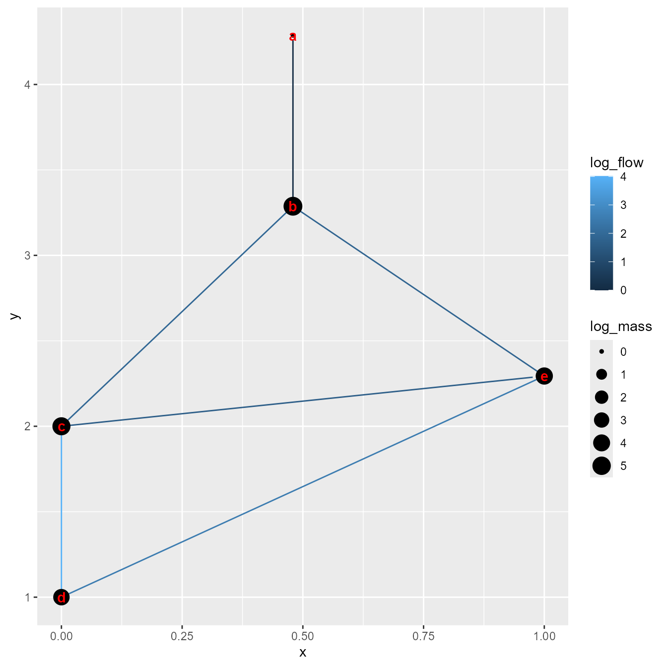
We can then plot the estimated foodweb:

# Plot foodweb at equilibrium
# using pelagic producers as x-axis and trophic level as y-axis
plot_foodweb( out$rep$out_initial$Qe_ij,  
              xtracer_i = ifelse(taxa_to_include=="Krill",1,0),
              B_i = out$rep$out_initial$B_i,
              type_i = type_i[taxa_to_include] )
#> Warning: Removed 4 rows containing missing values or values outside the scale range
#> (`geom_point()`).

Runtime for this vignette: 3.09 mins

James Thorson

Eastern Bering Sea