Fits a dynamic structural equation model
Usage
dsem(
  sem,
  tsdata,
  family = Map(function(.) fixed(), colnames(tsdata)),
  estimate_delta0 = FALSE,
  estimate_mu = NULL,
  prior_negloglike = NULL,
  control = dsem_control(),
  covs = colnames(tsdata)
)
Arguments
- sem
Specification for time-series structural equation model structure including lagged or simultaneous effects. See Details section in
make_dsem_ramfor more description- tsdata
time-series data, as outputted using
ts, withNAfor missing values.- family
A named list of families, each returning a class
family, includingfixed(),gaussian(),binomial(),Gamma(),poisson(),lognormal(),tweedie(), orgaussian_fixed_sd()with names that match levels ofcolnames(tsdata)to allow different families by variable. Familyfixed()specifies that states are known (i.e., measurements for that variable have no error). Other families allow users to supply a link function includingidentity,log,logit, orcloglog. For examplefamily = list(y = binomial("logit"), x = fixed())would specify logit-linked Bernoulli distribution for variabletsdata$yand a fixed (no measurement error) distribution fortsdata$x. For many variables, it is convenient to do e.g.,family = Map(function(.) gaussian(), colnames(tsdata))rather than writing them all manually.- estimate_delta0
Boolean indicating whether to estimate deviations from equilibrium in initial year as fixed effects, or alternatively to assume that dynamics start at some stochastic draw away from the stationary distribution
- estimate_mu
character-vector listing columns of
tsdatafor which to estimate the mean, which is subtracted off oftsdataprior to evaluating interactions among parameters. The defaultestimate_mu = NULLestimates the mean for every column with at least one value that is notNA(i.e., does not estimate the mean for latent variables). If you want to have nomuparameters, useestimate_mu = vector().- prior_negloglike
A user-provided function that takes as input the vector of fixed effects out$obj$par returns the negative log-prior probability. For example
prior_negloglike = function(obj) -1 * dnorm( obj$par[1], mean=0, sd=0.1, log=TRUE)specifies a normal prior probability for the for the first fixed effect with mean of zero and logsd of 0.1. NOTE: this implementation does not work well withtmbstanand is highly experimental. Note that the user must load RTMB usinglibrary(RTMB)prior to running the model.- control
Output from
dsem_control, used to define user settings, and see documentation for that function for details.- covs
optional: a character vector of one or more elements, with each element giving a string of variable names, separated by commas. Variances and covariances among all variables in each such string are added to the model. Warning: covs="x1, x2" and covs=c("x1", "x2") are not equivalent: covs="x1, x2" specifies the variance of x1, the variance of x2, and their covariance, while covs=c("x1", "x2") specifies the variance of x1 and the variance of x2 but not their covariance. These same covariances can be added manually via argument
sem, but using argumentcovsmight save time for models with many variables.
Value
An object (list) of class dsem. Elements include:
- obj
TMB object from
MakeADFun- ram
RAM parsed by
make_dsem_ram- model
SEM structure parsed by
make_dsem_ramas intermediate description of model linkages- tmb_inputs
The list of inputs passed to
MakeADFun- opt
The output from
nlminb- sdrep
The output from
sdreport- interal
Objects useful for package function, i.e., all arguments passed during the call
- run_time
Total time to run model
Details
A DSEM involves (at a minimum):
- Time series
a matrix \(\mathbf X\) where column \(\mathbf x_c\) for variable c is a time-series;
- Path diagram
a user-supplied specification for the path coefficients, which define the precision (inverse covariance) \(\mathbf Q\) for a matrix of state-variables and see
make_dsem_ramfor more details on the math involved.
The model also estimates the time-series mean \( \mathbf{\mu}_c \) for each variable. The mean and precision matrix therefore define a Gaussian Markov random field for \(\mathbf X\):
$$ \mathrm{vec}(\mathbf X) \sim \mathrm{MVN}( \mathrm{vec}(\mathbf{I_T} \otimes \mathbf{\mu}), \mathbf{Q}^{-1}) $$
Users can the specify
a distribution for measurement errors (or assume that variables are measured without error) using
argument family. This defines the link-function \(g_c(.)\) and distribution \(f_c(.)\)
for each time-series \(c\):
$$ y_{t,c} \sim f_c( g_c^{-1}( x_{t,c} ), \theta_c )$$
dsem then estimates all specified coefficients, time-series means \(\mu_c\), and distribution
measurement errors \(\theta_c\) via maximizing a log-marginal likelihood, while
also estimating state-variables \(x_{t,c}\).
summary.dsem then assembles estimates and standard errors in an easy-to-read format.
Standard errors for fixed effects (path coefficients, exogenoux variance parameters, and measurement error parameters)
are estimated from the matrix of second derivatives of the log-marginal likelihod,
and standard errors for random effects (i.e., missing or state-space variables) are estimated
from a generalization of this method (see sdreport for details).
Latent variables
Any column \(\mathbf x_c\) of tsdata that includes only NA values
represents a latent variable, and all others are called manifest variables.
The identifiability criteria for latent variables
can be complicated. To explain, we ignore lagged effects (only simultaneous paths)
and classify three types of latent variables:
- factor latent variables:
any latent variable \(\mathbf F\) that includes paths out from it to manifest variables, but has no paths from manifest variables into \(\mathbf F\) is a factor variable. These are identifable by fixing their SD (i.e., at one), and using a trimmed Cholesky parameterization (i.e., each successive factor includes fewer paths to manifest variables). See the DFA vignette for an example. Factor latent variables can be used to represent residual covariance while also estimating the source of that covariance explicitly
- intermediate latent variables:
Any latent variable \(\mathbf Y\) that includes paths in from some manifest variables \(\mathbf X\) and some paths out to manifest variables \(\mathbf Z\) is an intermediate latent variable. In general, the at least one path in or out must be fixed a priori (e.g., at one) to identify the scale of the intermediate LV. These intermediate latent variables can represent ecological concepts that serve as intermediate link between different manifest variables
- composite latent variables:
Any latent variable \(\mathbf C\) that includes paths in from some manifest variables \(\mathbf X\) and no paths out to manifest variables is a composite latent variable. In general, you must fix all paths to composite variables a priori, and must also fix the SD a priori (e.g., at zero). These composite variables allow DSEM to estimate a response with standard errors that integrates across multiple manifest variables
As stated, these criteria do not involve paths from one to another latent variable. These are also possible, but involve more complicated identifiability criteria.
When to do (ot not do) model selection
In general, DSEM can be used for predictive modelling and/or structural causal modelling.
For predictive modelling, DSEM provides an expressive
interface to specify any number of fixed effects and use these to represent the
covariance among variables and over time. The predictive error is expected to
decrease when using a parsimonious model, and model selection might be appropriate
using either stepwise_selection or some manual rule for dropping
coefficients that are not statistically significant using a likelihood ratio or
Wald test.
However, structural causal modelling (SCM) is necessary for models to be transferable
to new environments (patterns of colinearity), or for counterfactual analysis.
In general, SCM does not involve using parsimony as a basis for model selection.
Instead, SCM structure should be defined based on ecological knowledge, and
models can be further elaborated using tests of directional separation
(see test_dsep).
References
Introducing the package, its features, and comparison with other software (to cite when using dsem):
Thorson, J. T., Andrews, A., Essington, T., Large, S. (2024). Dynamic structural equation models synthesize ecosystem dynamics constrained by ecological mechanisms. Methods in Ecology and Evolution. doi:10.1111/2041-210X.14289
Introducing moderated DSEM (e.g., nonstationarity and varying paths):
Thorson, J. T., Kristensen, K. (In press). Ecological examples of nonstationarity, nonlinearity, and statistical interactions in dynamic structural equation models. Methods in Ecology and Evolution. https://ecoevorxiv.org/repository/view/11418/
Examples
# Define model
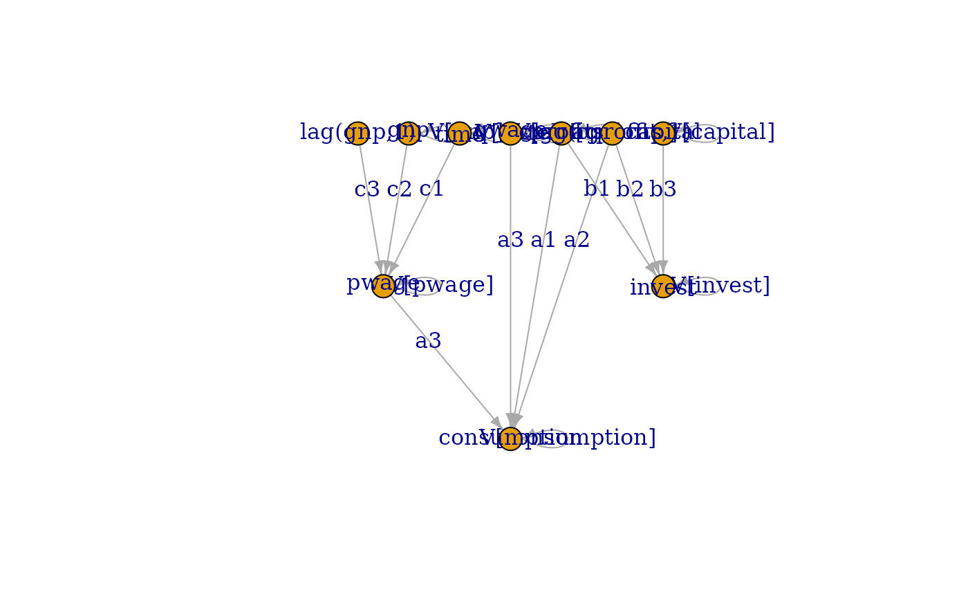
sem = "
# Link, lag, param_name
cprofits -> consumption, 0, a1
cprofits -> consumption, 1, a2
pwage -> consumption, 0, a3
gwage -> consumption, 0, a3
cprofits -> invest, 0, b1
cprofits -> invest, 1, b2
capital -> invest, 0, b3
gnp -> pwage, 0, c2
gnp -> pwage, 1, c3
time -> pwage, 0, c1
"
# Load data
data(KleinI, package="AER")
TS = ts(data.frame(KleinI, "time"=time(KleinI) - 1931))
tsdata = TS[,c("time","gnp","pwage","cprofits",'consumption',
"gwage","invest","capital")]
# Fit model
fit = dsem(
sem = sem,
tsdata = tsdata,
estimate_delta0 = TRUE,
control = dsem_control(quiet=TRUE)
)
summary( fit )
#> path lag name start parameter first
#> 1 cprofits -> consumption 0 a1 NA 1 cprofits
#> 2 cprofits -> consumption 1 a2 NA 2 cprofits
#> 3 pwage -> consumption 0 a3 NA 3 pwage
#> 4 gwage -> consumption 0 a3 NA 3 gwage
#> 5 cprofits -> invest 0 b1 NA 4 cprofits
#> 6 cprofits -> invest 1 b2 NA 5 cprofits
#> 7 capital -> invest 0 b3 NA 6 capital
#> 8 gnp -> pwage 0 c2 NA 7 gnp
#> 9 gnp -> pwage 1 c3 NA 8 gnp
#> 10 time -> pwage 0 c1 NA 9 time
#> 11 time <-> time 0 V[time] NA 10 time
#> 12 gnp <-> gnp 0 V[gnp] NA 11 gnp
#> 13 pwage <-> pwage 0 V[pwage] NA 12 pwage
#> 14 cprofits <-> cprofits 0 V[cprofits] NA 13 cprofits
#> 15 consumption <-> consumption 0 V[consumption] NA 14 consumption
#> 16 gwage <-> gwage 0 V[gwage] NA 15 gwage
#> 17 invest <-> invest 0 V[invest] NA 16 invest
#> 18 capital <-> capital 0 V[capital] NA 17 capital
#> second direction Estimate Std_Error z_value p_value
#> 1 consumption 1 0.19323185 0.08199229 2.356708 1.843776e-02
#> 2 consumption 1 0.08942112 0.08136334 1.099035 2.717530e-01
#> 3 consumption 1 0.79625663 0.03594118 22.154439 9.452934e-109
#> 4 consumption 1 0.79625663 0.03594118 22.154439 9.452934e-109
#> 5 invest 1 0.48138141 0.08740019 5.507785 3.633777e-08
#> 6 invest 1 0.33084616 0.09069261 3.647995 2.642950e-04
#> 7 invest 1 -0.11150752 0.02408258 -4.630214 3.652875e-06
#> 8 pwage 1 0.44041577 0.02921824 15.073314 2.426312e-51
#> 9 pwage 1 0.14476511 0.03370693 4.294817 1.748376e-05
#> 10 pwage 1 0.13029837 0.02882711 4.519995 6.184119e-06
#> 11 time 2 6.05530071 0.93435313 6.480741 9.127318e-11
#> 12 gnp 2 10.32020497 1.58102475 6.527542 6.685791e-11
#> 13 pwage 2 0.69302930 0.10701058 6.476269 9.401826e-11
#> 14 cprofits 2 4.10929046 0.63141034 6.508114 7.610017e-11
#> 15 consumption 2 0.92285232 0.14239896 6.480752 9.126683e-11
#> 16 gwage 2 1.90952975 0.29464666 6.480745 9.127100e-11
#> 17 invest 2 0.91015034 0.14046563 6.479523 9.201284e-11
#> 18 capital 2 9.67950590 1.49358015 6.480741 9.127332e-11
plot( fit )
 plot( fit, edge_label="value" )
