Description
FishLife is an R package for estimating evolutionary
trade-offs among traits for >34,000 described fishes. It also applies
phylogenetic trait imputation, i.e., is used to predict and reposit
predicted life-history parameters for all fishes, where imputed values
are informed by both life-history correlations and similarities among
related species. The package comes with three databases and pre-run
results:
- The database and results described by Thorson et al. (2023), introducing phylogenetic structural equation models and combining this with phylogenetic comparative methods to describe trade-offs among a larger set of life-history, morphometric, behavioral, trophic, and reproductive traits;
- The database and results described by Thorson (2020), applying phylogenetic factor analysis to the original database as well as RAM Legacy database records of stock-recruit relationships to estimate a full life-cycle model for all species;
- The original database and results described by Thorson Munch Cope Gao (2017), introducing phylogenetic factor analysis and using records of size, growth, maturity, and mortality parameters from FishBase as downloaded in 2016.
In this vignete, we show how to access output from these various models.
Thorson et al. 2023 results
Starting with Thorson et al. (2023), FishLife uses ape class
phylo to represent relatedness among taxa. This has several
benefits:
- It facilitates collaboration between evolutionary and ecological researchers for fishes;
- It represents relatedness based on evolutionary distance, rather than simply approximating relatedness based on taxonomy;
- It allows FishLife to use well-maintained dependencies to input(read, subset, and merge) or output (plot and tabulate) results.
However, this also results in changes in how results are accessed.
Although we provide a function
as(FishLife::FishBase_and_Morphometrics,"phylo4d"), we find
that it is too slow to be useful. Therefore, we instead recommend
searching for a taxon name manually. We demonstrate this for red
snapper:
edge_names = c( FishBase_and_Morphometrics$tree$tip.label,
                FishBase_and_Morphometrics$tree$node.label[-1] ) # Removing root

#
which_g = match( "Lutjanus campechanus", edge_names )
Table2023 = cbind(
  Mean = FishBase_and_Morphometrics$beta_gv[which_g,],
  SE = sqrt(diag(FishBase_and_Morphometrics$Cov_gvv[which_g,,]))
)
knitr::kable( Table2023, digits=3)| Mean | SE | |
|---|---|---|
| log(age_max) | 3.573 | 0.136 |
| trophic_level | 4.133 | 0.323 |
| log(aspect_ratio) | 0.614 | 0.140 |
| log(fecundity) | 15.976 | 0.518 |
| log(growth_coefficient) | -1.863 | 0.111 |
| temperature | 23.815 | 0.730 |
| log(length_max) | 4.451 | 0.090 |
| log(length_infinity) | 4.546 | 0.046 |
| log(length_maturity) | 3.526 | 0.126 |
| log(age_maturity) | 1.175 | 0.231 |
| log(natural_mortality) | -1.420 | 0.123 |
| log(weight_infinity) | 9.415 | 0.145 |
| log(max_body_depth) | -0.038 | 0.010 |
| log(max_body_width) | -0.895 | 0.010 |
| log(lower_jaw_length) | -0.874 | 0.010 |
| log(min_caudal_pedoncule_depth) | -1.230 | 0.010 |
| log(offspring_size) | -0.234 | 0.150 |
| base | 0.906 | 0.244 |
| spawning_typeguarders | 0.035 | 0.140 |
| spawning_typebearers | 0.058 | 0.202 |
| base | 0.109 | 0.151 |
| habitatbathymetric | 0.043 | 0.138 |
| habitatbenthopelagic | 0.026 | 0.081 |
| habitatreefassociated | 0.786 | 0.258 |
| habitatpelagic | 0.036 | 0.123 |
| base | 0.019 | 0.029 |
| feeding_modemacrofauna | 0.944 | 0.159 |
| feeding_modeplanktivorous_or_other | 0.037 | 0.154 |
| base | 0.859 | 0.234 |
| body_shapeelongated | 0.025 | 0.081 |
| body_shapeshort_and_or_deep | 0.068 | 0.153 |
| body_shapeeellike | 0.035 | 0.146 |
| body_shapeother | 0.013 | 0.096 |
Thorson 2020 results
The Thorson (2020) analysis sought to maintain customized code for accessing and plotting results. We again demonstrate this for red snapper, which is within the FishBase database used to train the model so its predictions are relatively precise.
# Get basic plot for Lutjanus campechanus
Taxa = Search_species( Genus = "Lutjanus",
                       Species = "campechanus")$match_taxonomy
Predict = Plot_taxa( Taxa,
                     mfrow=c(3,2) )
#>      [,1]           [,2]
#> [1,] "K"            "M"
#> [2,] "Winfinity"    "Loo"
#> [3,] "tmax"         "tm"
#> [4,] "Lm"           "Temperature"
#> [5,] "ln_margsd"    "rho"
#> [6,] "logitbound_h" "ln_r"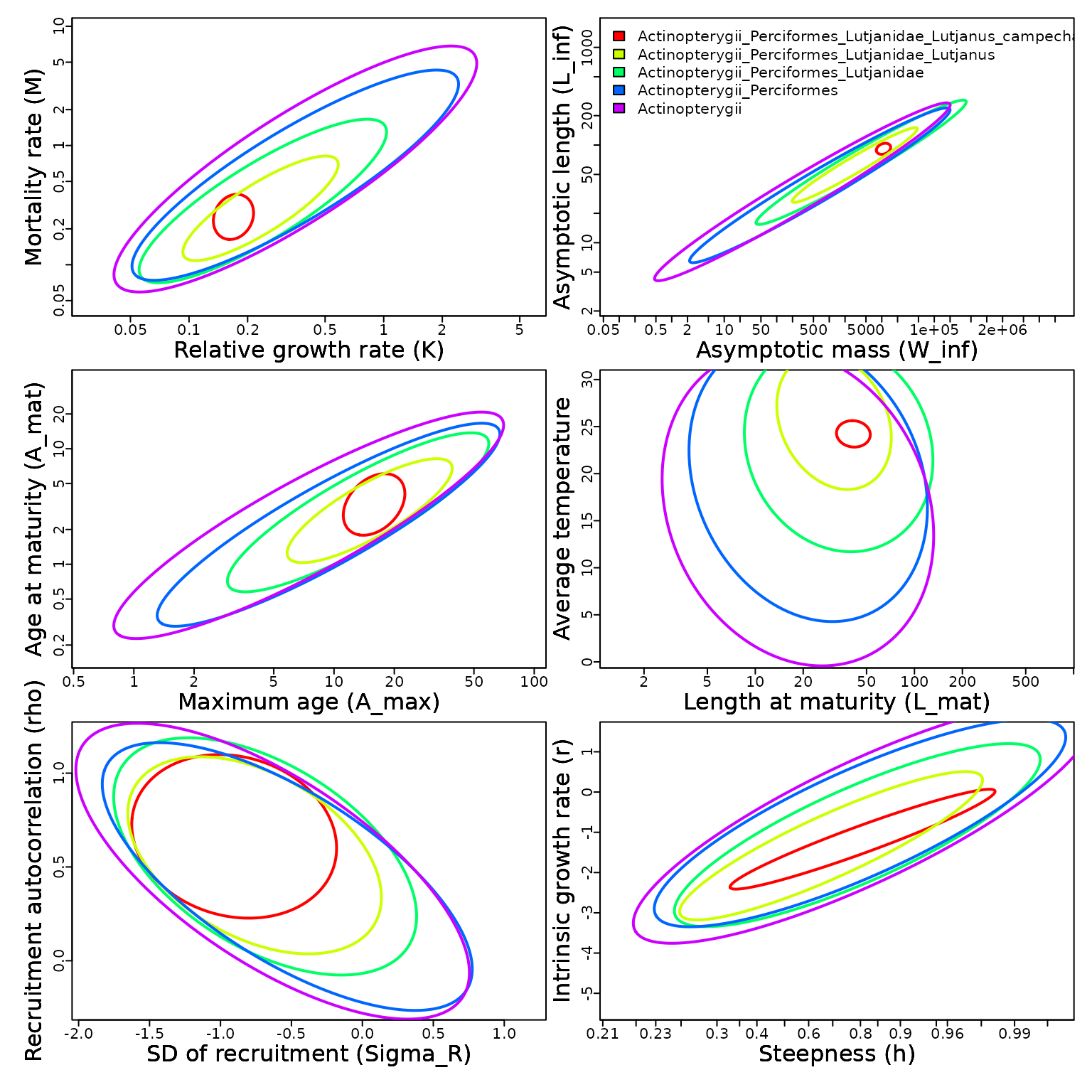
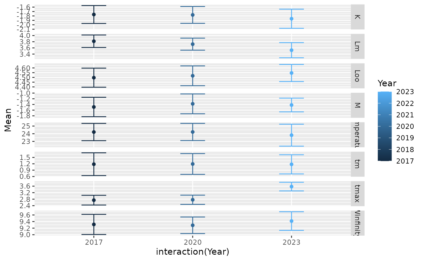
We then show updated values for the predictive mean and standard errors…
| Mean | SE | |
|---|---|---|
| Loo | 4.517 | 0.053 |
| K | -1.777 | 0.097 |
| Winfinity | 9.287 | 0.128 |
| tmax | 2.763 | 0.145 |
| tm | 1.192 | 0.250 |
| M | -1.378 | 0.178 |
| Lm | 3.722 | 0.100 |
| Temperature | 24.230 | 0.573 |
| ln_var | -2.556 | 0.821 |
| rho | 0.663 | 0.178 |
| ln_MASPS | 1.223 | 1.172 |
| ln_margsd | -0.904 | 0.295 |
| h | 0.770 | 0.157 |
| logitbound_h | 1.143 | 1.149 |
| ln_Fmsy_over_M | 1.089 | 0.730 |
| ln_Fmsy | -0.288 | 0.767 |
| ln_r | -1.171 | 0.507 |
| r | 0.348 | 0.158 |
| ln_G | 2.298 | 0.129 |
| G | 10.040 | 1.300 |
where Predict[[1]]$Mean_pred provides mean values, and
Predict[[1]]$Cov_pred provides the predictive covariance
for life-history parameters.
Traits are in log-space except for Temperature,
generation time G and intrinsict growth rate
r. If an analyst wants to back-transform a trait that is
reported in log-space, thought should be given to whether an analyst
wants to use a predictive median or predictive mean. The predictive
median is calculated by expnoentiating log-space values, while a
predictive mean requires some bias-correction (perhaps based on a
lognormal assumption using the predictive variance). Finally generation
time G and intrinsict growth rate r are
calculated based on a nonlinear transformation of other traits using the
Euler-Lotka formula, and we therefore report the mean in either
log-space or natural space, obtained by sampling from the constituent
traits, calculating the values for each sample, and then computing the
mean of those calculations. Given this procedure, exponentiating
ln_G will not typically equal G and the same
holds for ln_r and r.
Data-poor: Cortez rockfish
Next we demonstrate cortez rockfish, which is not within the FishBase database used to train the model, so its predictions are relatively based on information from related species within genus Sebastes.
# Get basic plot for Sebastes cortezi
Taxa = Search_species( Genus = "Sebastes",
                       Species = "cortezi")$match_taxonomy
Predict = Plot_taxa( Taxa,
                     mfrow=c(3,2) )
#>      [,1]           [,2]
#> [1,] "K"            "M"
#> [2,] "Winfinity"    "Loo"
#> [3,] "tmax"         "tm"
#> [4,] "Lm"           "Temperature"
#> [5,] "ln_margsd"    "rho"
#> [6,] "logitbound_h" "ln_r"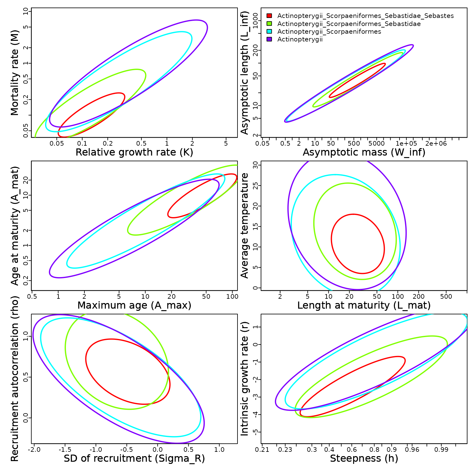
High-level: Scombridae
Third, we demonstrate predictions for family Scombridae, to show how predictions are available for higher-level taxonomies.
# Get basic plot for Family Scombridae
Plot_taxa( Search_species(Family="Scombridae")$match_taxonomy, mfrow=c(3,2) )
#>      [,1]           [,2]
#> [1,] "K"            "M"
#> [2,] "Winfinity"    "Loo"
#> [3,] "tmax"         "tm"
#> [4,] "Lm"           "Temperature"
#> [5,] "ln_margsd"    "rho"
#> [6,] "logitbound_h" "ln_r"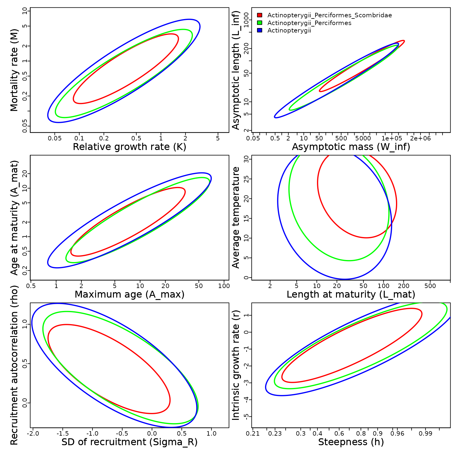
Comparison: Trouts
Fourth, we compare predictions for two species, brown and rainbow trout.
# Compare two species
Taxa = c( Search_species(Genus="Oncorhynchus",Species="mykiss",add_ancestors=FALSE)$match_taxonomy,
  Search_species(Genus="Salmo",Species="Trutta",add_ancestors=FALSE)$match_taxonomy )
Plot_taxa( Taxa, mfrow=c(3,2) )
#>      [,1]           [,2]
#> [1,] "K"            "M"
#> [2,] "Winfinity"    "Loo"
#> [3,] "tmax"         "tm"
#> [4,] "Lm"           "Temperature"
#> [5,] "ln_margsd"    "rho"
#> [6,] "logitbound_h" "ln_r"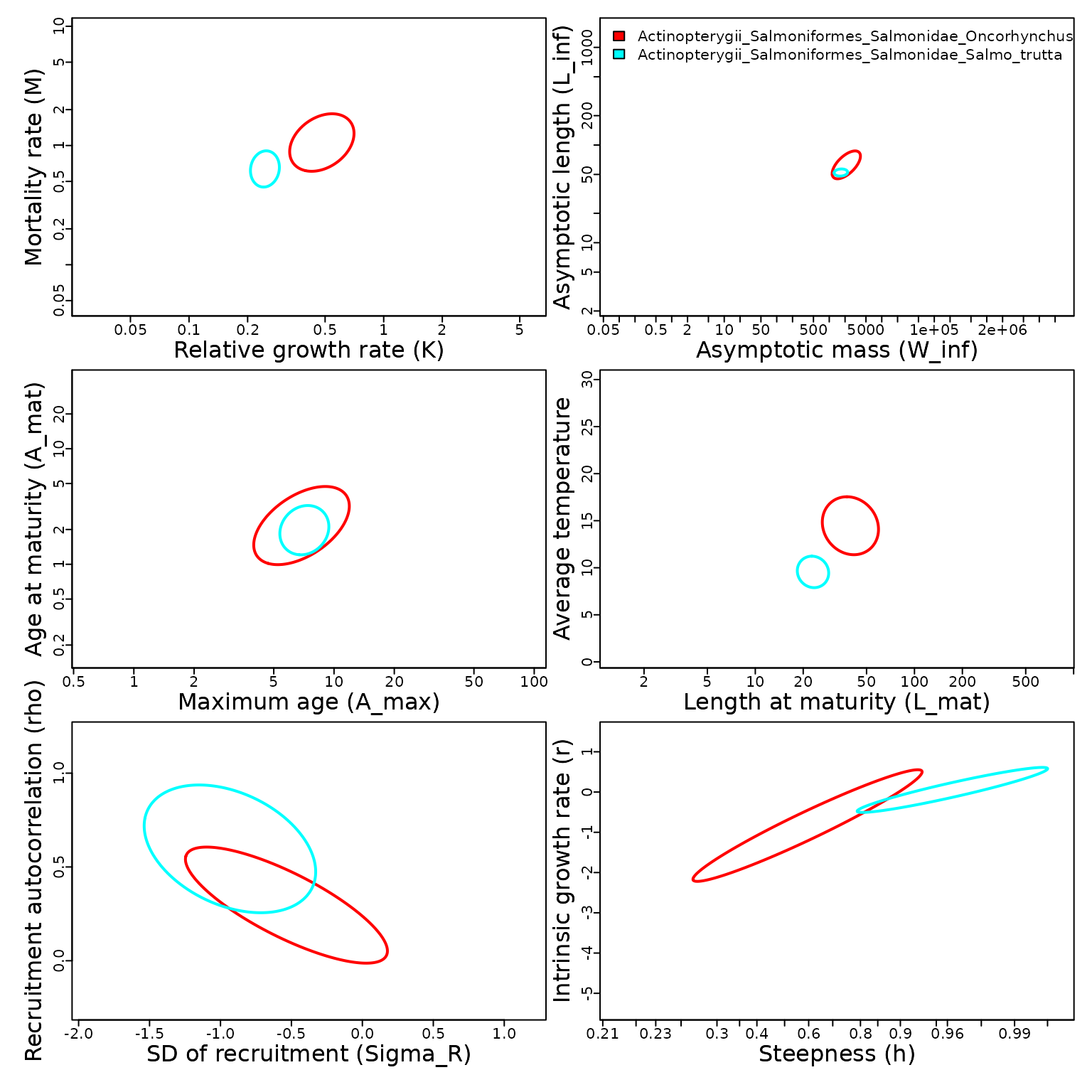
Thorson et al. (2017) results
Results from Thorson et al. (2017) are accessed similarly, but indicating the earlier database:
# Get basic plot for Lutjanus campechanus
Taxa = Search_species( Genus = "Lutjanus",
                       Species="campechanus",
                       Database = FishBase )$match_taxonomy
params = matrix( c( "Loo", "K", "Winfinity", "tmax",
                    "tm", "M", "Lm", "Temperature"), ncol=2 )
Predict = Plot_taxa( Taxa,
                     mfrow=c(2,2),
                     Database = FishBase,
                     params = params )
#>      [,1]        [,2]
#> [1,] "Loo"       "tm"
#> [2,] "K"         "M"
#> [3,] "Winfinity" "Lm"
#> [4,] "tmax"      "Temperature"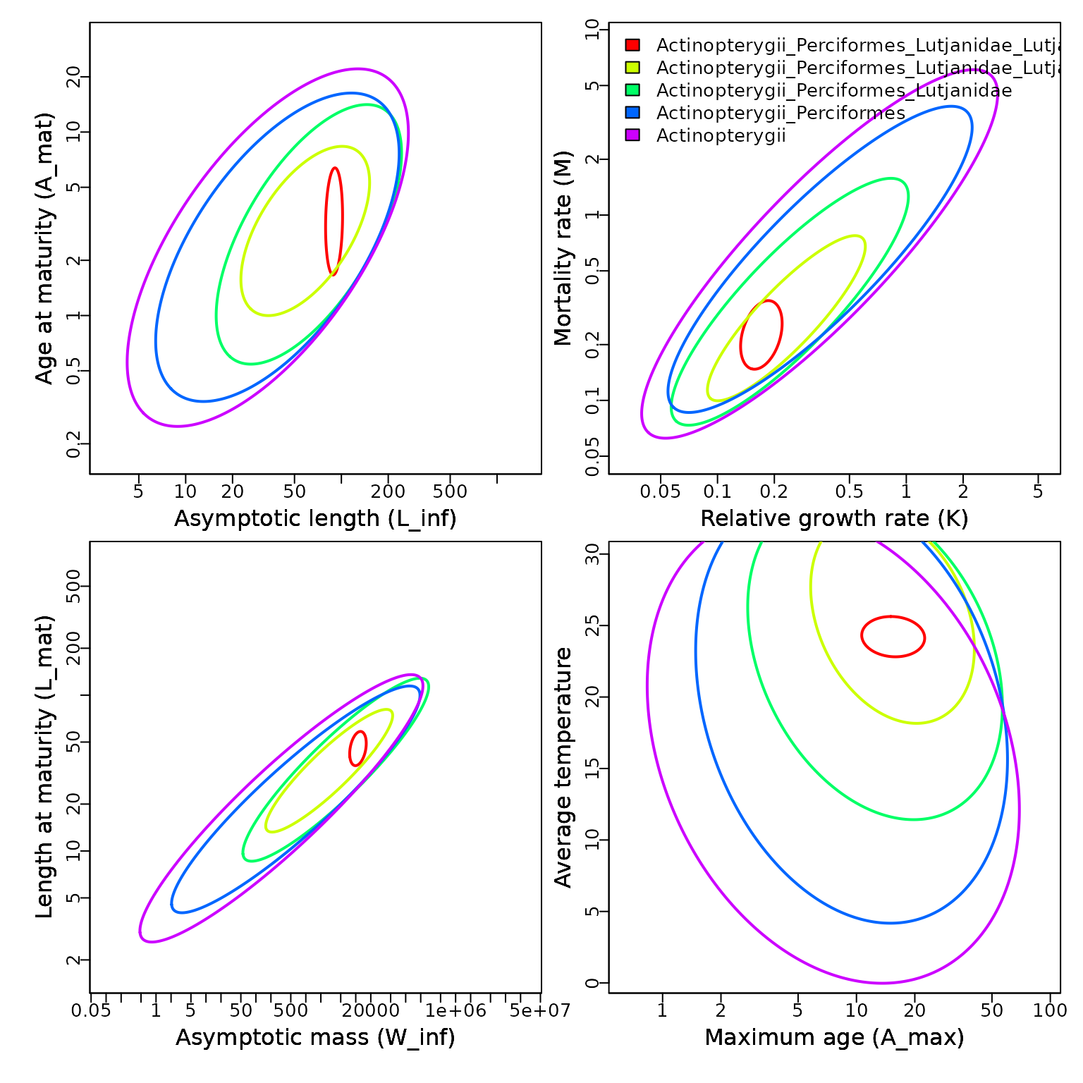
And we can again access the mean predicted values:
| Mean | SE | |
|---|---|---|
| Loo | 4.497 | 0.051 |
| K | -1.768 | 0.103 |
| Winfinity | 9.313 | 0.156 |
| tmax | 2.739 | 0.153 |
| tm | 1.181 | 0.274 |
| M | -1.489 | 0.174 |
| Lm | 3.816 | 0.103 |
| Temperature | 24.221 | 0.575 |
