Comparison with phylolm
We first compare syntax and run-times using simulated data against
phylolm. This confirms that runtimes from
phylosem are within an order of magnitude and that results
are nearly identical for BM, OU, delta, and kappa models.
# Settings
Ntree = 100
sd_x = 0.3
sd_y = 0.3
b0_x = 1
b0_y = 0
b_xy = 1

# Simulate tree
set.seed(1)
tree = ape::rtree(n=Ntree)

# Simulate data
x = b0_x + sd_x * phylolm::rTrait(n = 1, phy=tree)
ybar = b0_y + b_xy*x
y_normal = ybar + sd_y * phylolm::rTrait(n = 1, phy=tree)

# Construct, re-order, and reduce data
Data = data.frame(x=x,y=y_normal)[]

# Compare using BM model
start_time = Sys.time()
plm_bm = phylolm::phylolm(y ~ 1 + x, data=Data, phy=tree, model="BM" )
Sys.time() - start_time
#> Time difference of 0.003690243 secs
knitr::kable(summary(plm_bm)$coefficients, digits=3)
| (Intercept) |
-0.371 |
0.214 |
-1.734 |
0.086 |
| x |
1.117 |
0.101 |
11.053 |
0.000 |
| NA |
Intercept_x |
1.087 |
0.183 |
5.945 |
0.000 |
| NA |
Intercept_y |
-0.371 |
0.213 |
1.743 |
0.081 |
| x -> y |
p |
1.117 |
0.101 |
11.109 |
0.000 |
| x <-> x |
V[x] |
0.315 |
0.022 |
14.072 |
0.000 |
| y <-> y |
V[y] |
0.315 |
0.022 |
14.072 |
0.000 |
# Compare using OU
start_time = Sys.time()
plm_ou = phylolm::phylolm(y ~ 1 + x, data=Data, phy=tree, model="OUrandomRoot" )
Sys.time() - start_time
#> Time difference of 0.01382709 secs

start_time = Sys.time()
psem_ou = phylosem( sem = "x -> y, p",
          data = Data,
          tree = tree,
          estimate_ou = TRUE,
          control = phylosem_control(quiet = TRUE) )
Sys.time() - start_time
#> Time difference of 0.1069336 secs

knitr::kable(summary(psem_ou)$coefficients, digits=3)
| NA |
Intercept_x |
1.028 |
0.208 |
4.946 |
0.000 |
| NA |
Intercept_y |
-0.274 |
0.235 |
1.165 |
0.244 |
| x -> y |
p |
1.099 |
0.101 |
10.887 |
0.000 |
| x <-> x |
V[x] |
0.332 |
0.026 |
12.712 |
0.000 |
| y <-> y |
V[y] |
0.332 |
0.026 |
12.860 |
0.000 |
| (Intercept) |
-0.781 |
0.389 |
-2.006 |
0.048 |
| x |
1.095 |
0.101 |
10.850 |
0.000 |
knitr::kable(c( "phylolm_alpha"=plm_ou$optpar,
                "phylosem_alpha"=exp(psem_ou$parhat$lnalpha) ), digits=3)
| phylolm_alpha |
0.120 |
| phylosem_alpha |
0.105 |
# Compare using Pagel's lambda
start_time = Sys.time()
plm_lambda = phylolm::phylolm(y ~ 1 + x, data=Data, phy=tree, model="lambda" )
Sys.time() - start_time
#> Time difference of 0.02187824 secs

start_time = Sys.time()
psem_lambda = phylosem( sem = "x -> y, p",
          data = Data,
          tree = tree,
          estimate_lambda = TRUE,
          control = phylosem_control(quiet = TRUE) )
Sys.time() - start_time
#> Time difference of 0.07745767 secs

knitr::kable(summary(psem_lambda)$coefficients, digits=3)
| NA |
Intercept_x |
1.092 |
0.162 |
6.740 |
0.000 |
| NA |
Intercept_y |
-0.346 |
0.200 |
1.726 |
0.084 |
| x -> y |
p |
1.092 |
0.103 |
10.559 |
0.000 |
| x <-> x |
V[x] |
0.284 |
0.025 |
11.367 |
0.000 |
| y <-> y |
V[y] |
0.290 |
0.024 |
11.897 |
0.000 |
| (Intercept) |
-0.356 |
0.207 |
-1.718 |
0.089 |
| x |
1.102 |
0.103 |
10.744 |
0.000 |
knitr::kable(c( "phylolm_lambda"=plm_lambda$optpar,
                "phylosem_lambda"=plogis(psem_lambda$parhat$logitlambda) ), digits=3)
| phylolm_lambda |
0.980 |
| phylosem_lambda |
0.957 |
# Compare using Pagel's kappa
start_time = Sys.time()
plm_kappa = phylolm::phylolm(y ~ 1 + x, data=Data, phy=tree, model="kappa", lower.bound = 0, upper.bound = 3 )
Sys.time() - start_time
#> Time difference of 0.005553961 secs

start_time = Sys.time()
psem_kappa = phylosem( sem = "x -> y, p",
          data = Data,
          tree = tree,
          estimate_kappa = TRUE,
          control = phylosem_control(quiet = TRUE) )
Sys.time() - start_time
#> Time difference of 0.07955742 secs

knitr::kable(summary(psem_kappa)$coefficients, digits=3)
| NA |
Intercept_x |
1.078 |
0.186 |
5.783 |
0.000 |
| NA |
Intercept_y |
-0.368 |
0.216 |
1.705 |
0.088 |
| x -> y |
p |
1.113 |
0.101 |
11.025 |
0.000 |
| x <-> x |
V[x] |
0.299 |
0.029 |
10.183 |
0.000 |
| y <-> y |
V[y] |
0.300 |
0.029 |
10.343 |
0.000 |
| (Intercept) |
-0.370 |
0.216 |
-1.716 |
0.089 |
| x |
1.115 |
0.101 |
11.015 |
0.000 |
knitr::kable(c( "phylolm_kappa"=plm_kappa$optpar,
                "phylosem_kappa"=exp(psem_kappa$parhat$lnkappa) ), digits=3)
| phylolm_kappa |
0.930 |
| phylosem_kappa |
0.857 |
Generalized linear models
We also compare results among software for fitting phylogenetic
generalized linear models (PGLM).
Poisson-distributed response
First, we specifically explore a Poisson-distributed PGLM, comparing
phylosem against phylolm::phyloglm (which uses
Generalized Estimating Equations) and phyr::pglmm_compare
(which uses maximum likelihood).
# Settings
Ntree = 100
sd_x = 0.3
sd_y = 0.3
b0_x = 1
b0_y = 0
b_xy = 1

# Simulate tree
set.seed(1)
tree = ape::rtree(n=Ntree)

# Simulate data
x = b0_x + sd_x * phylolm::rTrait(n = 1, phy=tree)
ybar = b0_y + b_xy*x
y_normal = ybar + sd_y * phylolm::rTrait(n = 1, phy=tree)
y_pois = rpois( n=Ntree, lambda=exp(y_normal) )

# Construct, re-order, and reduce data
Data = data.frame(x=x,y=y_pois)

# Compare using phylolm::phyloglm
pglm = phylolm::phyloglm(y ~ 1 + x, data=Data, phy=tree, method="poisson_GEE" )
knitr::kable(summary(pglm)$coefficients, digits=3)
| (Intercept) |
-1.098 |
0.633 |
-1.736 |
0.083 |
| x |
1.314 |
0.247 |
5.320 |
0.000 |
#
pglmm = phyr::pglmm_compare(
  y ~ 1 + x,
  family = "poisson",
  data = Data,
  phy = tree )
#> Warning: the 'nobars' function has moved to the reformulas package. Please
#> update your imports, or ask an upstream package maintainer to do so.
knitr::kable(summary(pglmm), digits=3)
#> Generalized linear mixed model for poisson data fit by restricted maximum likelihood
#>
#> Call:y ~ 1 + x
#>
#> logLik    AIC    BIC
#> -173.4  354.7  360.6
#>
#> Phylogenetic random effects variance (s2):
#>    Variance Std.Dev
#> s2  0.06152   0.248
#>
#> Fixed effects:
#>                Value Std.Error  Zscore    Pvalue
#> (Intercept) -0.57006   0.30465 -1.8712   0.06132 .
#> x            1.18134   0.19805  5.9650 2.447e-09 ***
#> ---
#> Signif. codes:  0 '***' 0.001 '**' 0.01 '*' 0.05 '.' 0.1 ' ' 1
| NA |
Intercept_x |
1.087 |
0.183 |
5.945 |
0.000 |
| NA |
Intercept_y |
-0.581 |
0.305 |
1.904 |
0.057 |
| x -> y |
p |
1.190 |
0.199 |
5.971 |
0.000 |
| x <-> x |
V[x] |
0.315 |
0.022 |
14.072 |
0.000 |
| y <-> y |
V[y] |
0.232 |
0.054 |
4.310 |
0.000 |
We also compare results against brms (which fits a
Bayesian hierarchical model), although we load results from compiled run
of brms to avoid users having to install STAN to run
vignettes for phylosem:
# Comare using Bayesian implementation in brms
library(brms)
Amat <- ape::vcv.phylo(tree)
Data$tips <- rownames(Data)
mcmc <- brm(
  y ~ 1 + x + (1 | gr(tips, cov = A)),
  data = Data, data2 = list(A = Amat),
  family = 'poisson',
  cores = 4
)
knitr::kable(fixef(mcmc), digits = 3)

# Plot them together
library(ggplot2)
pdat <- rbind.data.frame(
  coef(summary(pglm))[, 1:2],
  data.frame(Estimate = pglmm$B, StdErr = pglmm$B.se),
  setNames(as.data.frame(fixef(mcmc))[1:2], c('Estimate', 'StdErr')),
  setNames(summary(pgsem)$coefficients[2:3, 3:4], c('Estimate', 'StdErr'))
)
pdat$Param <- rep(c('Intercept', 'Slope'), 4)
pdat$Method <- rep( c('phylolm::phyloglm', 'phyr::pglmm_compare',
                     'brms::brm', 'phylosem::phylosem'), each = 2)
figure = ggplot(pdat, aes(
  x = Estimate, xmin = Estimate - StdErr,
  xmax = Estimate + StdErr, y = Param, color = Method
)) +
  geom_pointrange(position = position_dodge(width = 0.6)) +
  theme_classic() +
  theme(panel.grid.major.x = element_line(), panel.grid.minor.x = element_line())
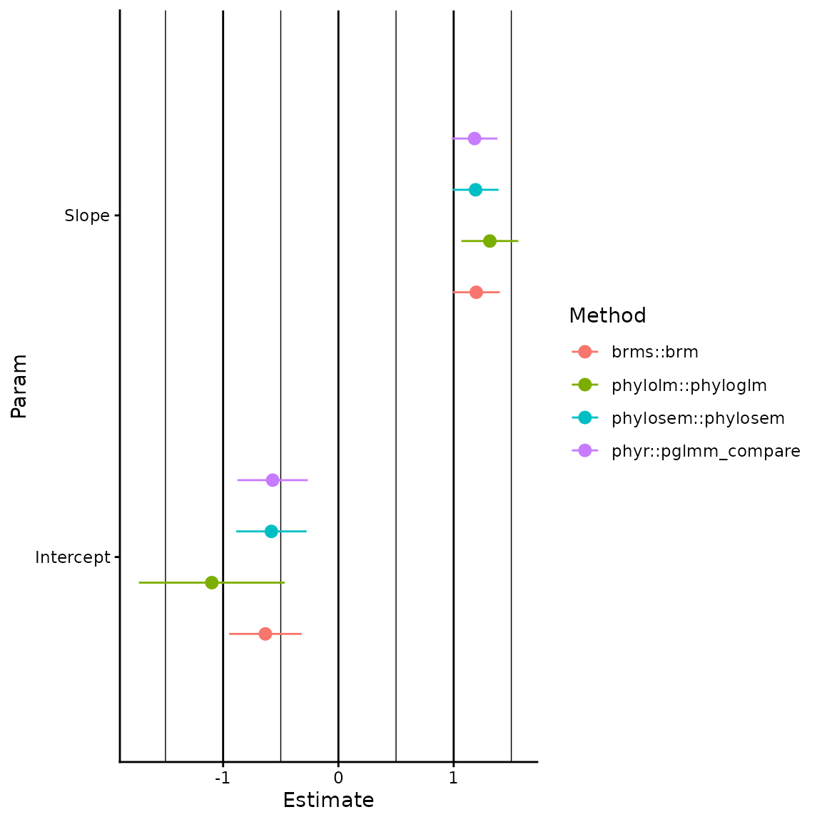
In this instance (and in others we have explored), results from
phylolm::phyloglm are generally different while those from
phylosem, phyr::pglmm_compare, and
brms are close but not quite identical.
Binomial regression
We also compare results for a Bernoulli-distributed response using
PGLM. We again compare phylosem against
phyr::pglmm_compare, and do not explore threshold models
which we expect to give different results due differences in assumptions
about how latent variables affect measurements.
# Settings
Ntree = 100
sd_x = 0.3
sd_y = 0.3
b0_x = 1
b0_y = 0
b_xy = 1

# Simulate tree
set.seed(1)
tree = ape::rtree(n=Ntree)

# Simulate data
x = b0_x + sd_x * phylolm::rTrait(n = 1, phy=tree)
ybar = b0_y + b_xy*x
y_normal = ybar + sd_y * phylolm::rTrait(n = 1, phy=tree)
y_binom = rbinom( n=Ntree, size=1, prob=plogis(y_normal) )

# Construct, re-order, and reduce data
Data = data.frame(x=x,y=y_binom)

#
pglmm = phyr::pglmm_compare(
  y ~ 1 + x,
  family = "binomial",
  data = Data,
  phy = tree )
knitr::kable(summary(pglmm), digits=3)
#> Generalized linear mixed model for binomial data fit by restricted maximum likelihood
#>
#> Call:y ~ 1 + x
#>
#> logLik    AIC    BIC
#> -63.74 135.47 141.31
#>
#> Phylogenetic random effects variance (s2):
#>    Variance Std.Dev
#> s2   0.1217  0.3489
#>
#> Fixed effects:
#>               Value Std.Error Zscore Pvalue
#> (Intercept) 0.23181   0.60650 0.3822 0.7023
#> x           0.44615   0.45800 0.9741 0.3300
| NA |
Intercept_x |
1.087 |
0.183 |
5.945 |
0.000 |
| NA |
Intercept_y |
0.204 |
0.589 |
0.346 |
0.730 |
| x -> y |
p |
0.458 |
0.468 |
0.977 |
0.328 |
| x <-> x |
V[x] |
-0.315 |
0.022 |
14.072 |
0.000 |
| y <-> y |
V[y] |
0.290 |
0.284 |
1.020 |
0.308 |
In this instance, phylosem and
phyr::pglmm_compare give similar estimates and standard
errors for the slope term.
Summary of PGLM results
Based on these two comparisons, we conclude that phylosem provides an
interface for maximum-likelihood estimate of phylogenetic generalized
linear models (PGLM), and extends this class to include mixed data
(i.e., a combination of different measurement types), missing data, and
non-recursive structural linkages. However, we also encourage further
cross-testing of different software for fitting phylogenetic generalized
linear models.
Compare with phylopath
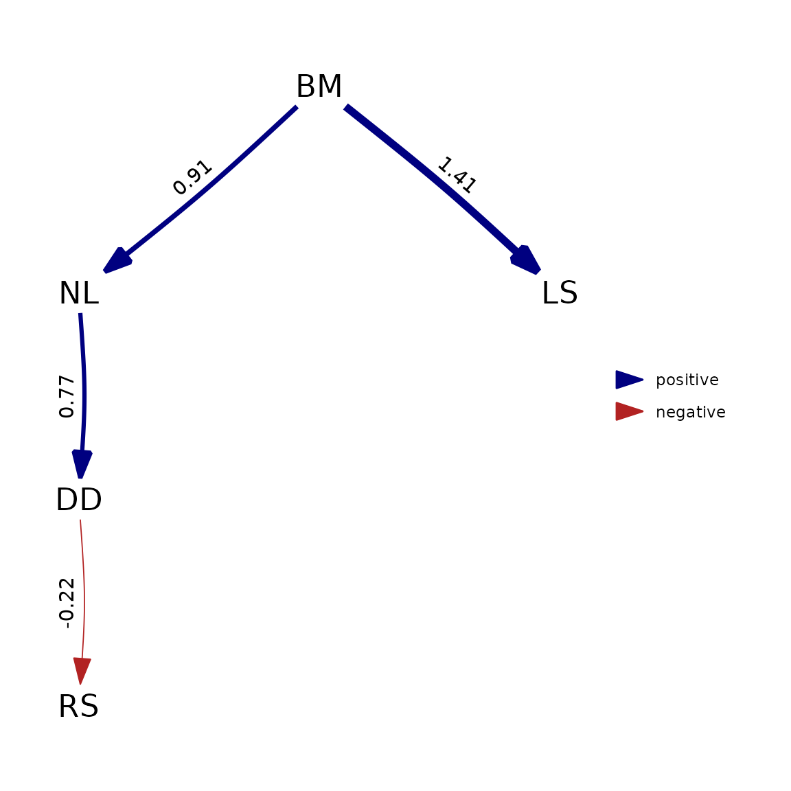
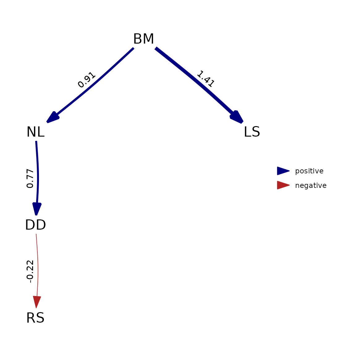
We next compare with a single run of phylopath. This
again confirms that runtimes are within an order of magnitude and
results are identical for standardized or unstandardized
coefficients.
library(phylopath)
library(phylosem)

# make copy of data that's rescaled
rhino_scaled = rhino
  rhino_scaled[,c("BM","NL","LS","DD","RS")] = scale(rhino_scaled[,c("BM","NL","LS","DD","RS")])

# Fit and plot using phylopath
dag <- DAG(RS ~ DD, LS ~ BM, NL ~ BM, DD ~ NL)
start_time = Sys.time()
result <- est_DAG( DAG = dag,
                    data = rhino,
                    tree = rhino_tree,
                    model = "BM",
                    measurement_error = FALSE )
Sys.time() - start_time
#> Time difference of 0.007565022 secs
plot(result)
# Fit and plot using phylosem
model = "
  DD -> RS, p1
  BM -> LS, p2
  BM -> NL, p3
  NL -> DD, p4
"
start_time = Sys.time()
psem = phylosem( sem = model,
          data = rhino_scaled[,c("BM","NL","DD","RS","LS")],
          tree = rhino_tree,
          control = phylosem_control(quiet = TRUE) )
Sys.time() - start_time
#> Time difference of 0.5466464 secs
plot( as_fitted_DAG(psem) )
#> Warning: Cannot determine which variables of this model are binary, so the scale of its coefficients is unknown.
#>   Paths into a binary variable are log odds ratios, while paths into a continuous variable are standardized regression coefficients.
#> ℹ This model was fitted by a version of phylopath older than 1.4.0, which did not record it. Refit it to label the coefficients, and to stop receiving this warning.
Comparison with sem
We next compare syntax and runtime against R-package
sem. This confirms that runtimes are within an order of
magnitude when specifying a star-phylogeny in phylosem to
match the assumed structure in sem
library(sem)
library(TreeTools)

# Simulation parameters
n_obs = 50
# Intercepts
a1 = 1
a2 = 2
a3 = 3
a4 = 4
# Slopes
b12 = 0.3
b23 = 0
b34 = 0.3
# Standard deviations
s1 = 0.1
s2 = 0.2
s3 = 0.3
s4 = 0.4

# Simulate data
E1 = rnorm(n_obs, sd=s1)
E2 = rnorm(n_obs, sd=s2)
E3 = rnorm(n_obs, sd=s3)
E4 = rnorm(n_obs, sd=s4)
Y1 = a1 + E1
Y2 = a2 + b12*Y1 + E2
Y3 = a3 + b23*Y2 + E3
Y4 = a4 + b34*Y3 + E4
Data = data.frame(Y1=Y1, Y2=Y2, Y3=Y3, Y4=Y4)

# Specify path diagram (in this case, using correct structure)
equations = "
  Y2 = b12 * Y1
  Y4 = b34 * Y3
"
model <- specifyEquations(text=equations, exog.variances=TRUE, endog.variances=TRUE)

# Fit using package:sem
start_time = Sys.time()
Sem <- sem(model, data=Data)
Sys.time() - start_time
#> Time difference of 0.006618261 secs

# Specify star phylogeny
tree_null = TreeTools::StarTree(n_obs)
  tree_null$edge.length = rep(1,nrow(tree_null$edge))
  rownames(Data) = tree_null$tip.label

# Fit using phylosem
start_time = Sys.time()
psem = phylosem( data = Data,
          sem = equations,
          tree = tree_null,
          control = phylosem_control(quiet = TRUE) )
Sys.time() - start_time
#> Time difference of 0.0262475 secs
We then compare estimated values for standardized coefficients
| Y1 -> Y2 |
Y1 |
Y2 |
b12 |
0.345 |
NA |
| Y3 -> Y4 |
Y3 |
Y4 |
b34 |
0.343 |
NA |
and also compare values for unstandardized coefficients:
| b12 |
0.660 |
| b34 |
0.390 |
| V[Y1] |
0.010 |
| V[Y2] |
0.038 |
| V[Y3] |
0.098 |
| V[Y4] |
0.126 |
| Y1 -> Y2 |
Y1 |
Y2 |
b12 |
0.660 |
0.274 |
| Y3 -> Y4 |
Y3 |
Y4 |
b34 |
0.390 |
0.162 |
| Y1 <-> Y1 |
Y1 |
Y1 |
V[Y1] |
0.010 |
NA |
| Y2 <-> Y2 |
Y2 |
Y2 |
V[Y2] |
0.038 |
NA |
| Y3 <-> Y3 |
Y3 |
Y3 |
V[Y3] |
0.098 |
NA |
| Y4 <-> Y4 |
Y4 |
Y4 |
V[Y4] |
0.126 |
NA |
Comparison with Rphylopars
Finally, we compare syntax and runtime against R-package
Rphylopars. This confirms that we can impute identical
estimates using both packages, when specifying a full-rank covariance in
phylosem
We note that phylosem also allows parsimonious
representations of the trait covariance via the inputted SEM
structure.
library(Rphylopars)

# Format data, within no values for species t1
Data = rhino[,c("BM","NL","DD","RS","LS")]
  rownames(Data) = tree$tip.label
Data['t1',] = NA

# fit using phylopars
start_time = Sys.time()
pars <- phylopars( trait_data = cbind(species=rownames(Data),Data),
                  tree = tree,
                  pheno_error = FALSE,
                  phylo_correlated = TRUE,
                  pheno_correlated = FALSE)
Sys.time() - start_time
#> Time difference of 0.0582068 secs

# Display estimates for missing values
knitr::kable(cbind( "Estimate"=pars$anc_recon["t1",], "Var"=pars$anc_var["t1",] ), digits=3)
| BM |
1.266 |
1.941 |
| NL |
1.600 |
1.856 |
| DD |
2.301 |
1.708 |
| RS |
0.431 |
1.909 |
| LS |
1.083 |
1.347 |
# fit using phylosem
start_time = Sys.time()
psem = phylosem( data = Data,
                 tree = tree,
                 sem = "",
                 covs = "BM, NL, DD, RS, LS",
                 control = phylosem_control(quiet = TRUE) )
Sys.time() - start_time
#> Time difference of 0.3055508 secs

# Display estimates for missing values
knitr::kable(cbind(
  "Estimate"=as.list(psem$sdrep,"Estimate")$x_vj[ match("t1",tree$tip.label), ],
  "Var"=as.list(psem$sdrep,"Std. Error")$x_vj[ match("t1",tree$tip.label), ]^2
), digits=3)
| 1.266 |
1.941 |
| 1.600 |
1.856 |
| 2.301 |
1.708 |
| 0.431 |
1.910 |
| 1.083 |
1.347 |